Two-Bit History

Jekyll2024-06-17T18:16:18+00:00https://twobithistory.org/feed.xmlTwo-Bit HistoryA Jekyll blog about the history of computingHow the ARPANET Protocols Worked2021-03-08T00:00:00+00:002021-03-08T00:00:00+00:00https://twobithistory.org/2021/03/08/arpanet-protocolsThe ARPANET changed computing forever by proving that computers of wildly different manufacture could be connected using standardized protocols. In my post on the historical significance of the ARPANET, I mentioned a few of those protocols, but didn’t describe them in any detail. So I wanted to take a closer look at them. I also wanted to see how much of the design of those early protocols survives in the protocols we use today.

The ARPANET protocols were, like our modern internet protocols, organized into layers.1 The protocols in the higher layers ran on top of the protocols in the lower layers. Today the TCP/IP suite has five layers (the Physical, Link, Network, Transport, and Application layers), but the ARPANET had only three layers—or possibly four, depending on how you count them.

I’m going to explain how each of these layers worked, but first an aside about who built what in the ARPANET, which you need to know to understand why the layers were divided up as they were.

Some Quick Historical Context

The ARPANET was funded by the US federal government, specifically the Advanced Research Projects Agency within the Department of Defense (hence the name “ARPANET”). The US government did not directly build the network; instead, it contracted the work out to a Boston-based consulting firm called Bolt, Beranek, and Newman, more commonly known as BBN.

BBN, in turn, handled many of the responsibilities for implementing the network but not all of them. What BBN did was design and maintain a machine known as the Interface Message Processor, or IMP. The IMP was a customized Honeywell minicomputer, one of which was delivered to each site across the country that was to be connected to the ARPANET. The IMP served as a gateway to the ARPANET for up to four hosts at each host site. It was basically a router. BBN controlled the software running on the IMPs that forwarded packets from IMP to IMP, but the firm had no direct control over the machines that would connect to the IMPs and become the actual hosts on the ARPANET.

The host machines were controlled by the computer scientists that were the end users of the network. These computer scientists, at host sites across the country, were responsible for writing the software that would allow the hosts to talk to each other. The IMPs gave hosts the ability to send messages to each other, but that was not much use unless the hosts agreed on a format to use for the messages. To solve that problem, a motley crew consisting in large part of graduate students from the various host sites formed themselves into the Network Working Group, which sought to specify protocols for the host computers to use.

So if you imagine a single successful network interaction over the ARPANET, (sending an email, say), some bits of engineering that made the interaction successful were the responsibility of one set of people (BBN), while other bits of engineering were the responsibility of another set of people (the Network Working Group and the engineers at each host site). That organizational and logistical happenstance probably played a big role in motivating the layered approach used for protocols on the ARPANET, which in turn influenced the layered approach used for TCP/IP.

Okay, Back to the Protocols

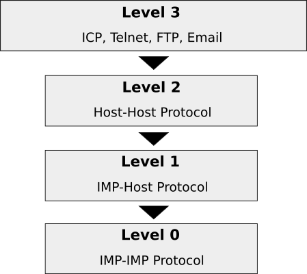The ARPANET protocol hierarchy.

The protocol layers were organized into a hierarchy. At the very bottom was “level 0.”2 This is the layer that in some sense doesn’t count, because on the ARPANET this layer was controlled entirely by BBN, so there was no need for a standard protocol. Level 0 governed how data passed between the IMPs. Inside of BBN, there were rules governing how IMPs did this; outside of BBN, the IMP sub-network was a black box that just passed on any data that you gave it. So level 0 was a layer without a real protocol, in the sense of a publicly known and agreed-upon set of rules, and its existence could be ignored by software running on the ARPANET hosts. Loosely speaking, it handled everything that falls under the Physical, Link, and Internet layers of the TCP/IP suite today, and even quite a lot of the Transport layer, which is something I’ll come back to at the end of this post.

The “level 1” layer established the interface between the ARPANET hosts and the IMPs they were connected to. It was an API, if you like, for the black box level 0 that BBN had built. It was also referred to at the time as the IMP-Host Protocol. This protocol had to be written and published because, when the ARPANET was first being set up, each host site had to write its own software to interface with the IMP. They wouldn’t have known how to do that unless BBN gave them some guidance.

The IMP-Host Protocol was specified by BBN in a lengthy document called [BBN
Report 1822](https://walden-family.com/impcode/BBN1822_Jan1976.pdf). The document was revised many times as the ARPANET evolved; what I’m going to describe here is roughly the way the IMP-Host protocol worked as it was initially designed. According to BBN’s rules, hosts could pass messages to their IMPs no longer than 8095 bits, and each message had a leader that included the destination host number and something called a link number.3 The IMP would examine the designation host number and then dutifully forward the message into the network. When messages were received from a remote host, the receiving IMP would replace the destination host number with the source host number before passing it on to the local host. Messages were not actually what passed between the IMPs themselves—the IMPs broke the messages down into smaller packets for transfer over the network—but that detail was hidden from the hosts.

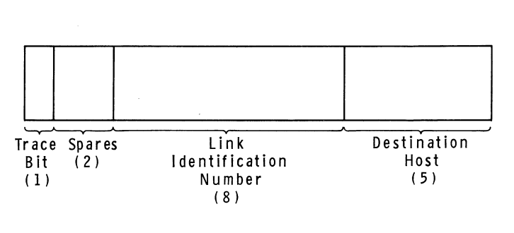The Host-IMP message leader format, as of 1969. Diagram from BBN Report_ _1763.

The link number, which could be any number from 0 to 255, served two purposes. It was used by higher level protocols to establish more than one channel of communication between any two hosts on the network, since it was conceivable that there might be more than one local user talking to the same destination host at any given time. (In other words, the link numbers allowed communication to be multiplexed between hosts.) But it was also used at the level 1 layer to control the amount of traffic that could be sent between hosts, which was necessary to prevent faster computers from overwhelming slower ones. As initially designed, the IMP-Host Protocol limited each host to sending just one message at a time over each link. Once a given host had sent a message along a link to a remote host, it would have to wait to receive a special kind of message called an RFNM (Request for Next Message) from the remote IMP before sending the next message along the same link. Later revisions to this system, made to improve performance, allowed a host to have up to eight messages in transit to another host at a given time.4

The “level 2” layer is where things really start to get interesting, because it was this layer and the one above it that BBN and the Department of Defense left entirely to the academics and the Network Working Group to invent for themselves. The level 2 layer comprised the Host-Host Protocol, which was first sketched in RFC 9 and first officially specified by RFC 54. A more readable explanation of the Host-Host Protocol is given in the [ARPANET Protocol
Handbook](http://mercury.lcs.mit.edu/~jnc/tech/arpaprot.html).

The Host-Host Protocol governed how hosts created and managed connections with each other. A connection was a one-way data pipeline between a write socket on one host and a read socket on another host. The “socket” concept was introduced on top of the limited level-1 link facility (remember that the link number can only be one of 256 values) to give programs a way of addressing a particular process running on a remote host. Read sockets were even-numbered while write sockets were odd-numbered; whether a socket was a read socket or a write socket was referred to as the socket’s gender. There were no “port numbers” like in TCP. Connections could be opened, manipulated, and closed by specially formatted Host-Host control messages sent between hosts using link 0, which was reserved for that purpose. Once control messages were exchanged over link 0 to establish a connection, further data messages could then be sent using another link number picked by the receiver.

Host-Host control messages were identified by a three-letter mnemonic. A connection was established when two hosts exchanged a STR (sender-to-receiver) message and a matching RTS (receiver-to-sender) message—these control messages were both known as Request for Connection messages. Connections could be closed by the CLS (close) control message. There were further control messages that changed the rate at which data messages were sent from sender to receiver, which were needed to ensure again that faster hosts did not overwhelm slower hosts. The flow control already provided by the level 1 protocol was apparently not sufficient at level 2; I suspect this was because receiving an RFNM from a remote IMP was only a guarantee that the remote IMP had passed the message on to the destination host, not that the host had fully processed the message. There was also an INR (interrupt-by-receiver) control message and an INS (interrupt-by-sender) control message that were primarily for use by higher-level protocols.

The higher-level protocols all lived in “level 3”, which was the Application layer of the ARPANET. The Telnet protocol, which provided a virtual teletype connection to another host, was perhaps the most important of these protocols, but there were many others in this level too, such as FTP for transferring files and various experiments with protocols for sending email.

One protocol in this level was not like the others: the Initial Connection Protocol (ICP). ICP was considered to be a level-3 protocol, but really it was a kind of level-2.5 protocol, since other level-3 protocols depended on it. ICP was needed because the connections provided by the Host-Host Protocol at level 2 were only one-way, but most applications required a two-way (i.e. full-duplex) connection to do anything interesting. ICP specified a two-step process whereby a client running on one host could connect to a long-running server process on another host. The first step involved establishing a one-way connection from the server to the client using the server process’ well-known socket number. The server would then send a new socket number to the client over the established connection. At that point, the existing connection would be discarded and two new connections would be opened, a read connection based on the transmitted socket number and a write connection based on the transmitted socket number plus one. This little dance was a necessary prelude to most things—it was the first step in establishing a Telnet connection, for example.

That finishes our ascent of the ARPANET protocol hierarchy. You may have been expecting me to mention a “Network Control Protocol” at some point. Before I sat down to do research for this post and my last one, I definitely thought that the ARPANET ran on a protocol called NCP. The acronym is occasionally used to refer to the ARPANET protocols as a whole, which might be why I had that idea. RFC 801, for example, talks about transitioning the ARPANET from “NCP” to “TCP” in a way that makes it sound like NCP is an ARPANET protocol equivalent to TCP. But there has never been a “Network Control Protocol” for the ARPANET (even if [Encyclopedia Britannica
thinks so](https://www.britannica.com/topic/ARPANET)), and I suspect people have mistakenly unpacked “NCP” as “Network Control Protocol” when really it stands for “Network Control Program.” The Network Control Program was the kernel-level program running in each host responsible for handling network communication, equivalent to the TCP/IP stack in an operating system today. “NCP”, as it’s used in RFC 801, is a metonym, not a protocol.

A Comparison with TCP/IP

The ARPANET protocols were all later supplanted by the TCP/IP protocols (with the exception of Telnet and FTP, which were easily adapted to run on top of TCP). Whereas the ARPANET protocols were all based on the assumption that the network was built and administered by a single entity (BBN), the TCP/IP protocol suite was designed for an inter-net, a network of networks where everything would be more fluid and unreliable. That led to some of the more immediately obvious differences between our modern protocol suite and the ARPANET protocols, such as how we now distinguish between a Network layer and a Transport layer. The Transport layer-like functionality that in the ARPANET was partly implemented by the IMPs is now the sole responsibility of the hosts at the network edge.

What I find most interesting about the ARPANET protocols though is how so much of the transport-layer functionality now in TCP went through a janky adolescence on the ARPANET. I’m not a networking expert, so I pulled out my college networks textbook (Kurose and Ross, let’s go), and they give a pretty great outline of what a transport layer is responsible for in general. To summarize their explanation, a transport layer protocol must minimally do the following things. Here segment is basically equivalent to message as the term was used on the ARPANET:

• Provide a delivery service between processes and not just host machines (transport layer multiplexing and demultiplexing)
• Provide integrity checking on a per-segment basis (i.e. make sure there is no data corruption in transit)

A transport layer could also, like TCP does, provide reliable data transfer, which means:

• Segments are delivered in order
• No segments go missing
• Segments aren’t delivered so fast that they get dropped by the receiver (flow control)

It seems like there was some confusion on the ARPANET about how to do multiplexing and demultiplexing so that processes could communicate—BBN introduced the link number to do that at the IMP-Host level, but it turned out that socket numbers were necessary at the Host-Host level on top of that anyway. Then the link number was just used for flow control at the IMP-Host level, but BBN seems to have later abandoned that in favor of doing flow control between unique pairs of hosts, meaning that the link number started out as this overloaded thing only to basically became vestigial. TCP now uses port numbers instead, doing flow control over each TCP connection separately. The process-process multiplexing and demultiplexing lives entirely inside TCP and does not leak into a lower layer like on the ARPANET.

It’s also interesting to see, in light of how Kurose and Ross develop the ideas behind TCP, that the ARPANET started out with what Kurose and Ross would call a strict “stop-and-wait” approach to reliable data transfer at the IMP-Host level. The “stop-and-wait” approach is to transmit a segment and then refuse to transmit any more segments until an acknowledgment for the most recently transmitted segment has been received. It’s a simple approach, but it means that only one segment is ever in flight across the network, making for a very slow protocol—which is why Kurose and Ross present “stop-and-wait” as merely a stepping stone on the way to a fully featured transport layer protocol. On the ARPANET, “stop-and-wait” was how things worked for a while, since, at the IMP-Host level, a Request for Next Message had to be received in response to every outgoing message before any further messages could be sent. To be fair to BBN, they at first thought this would be necessary to provide flow control between hosts, so the slowdown was intentional. As I’ve already mentioned, the RFNM requirement was later relaxed for the sake of better performance, and the IMPs started attaching sequence numbers to messages and keeping track of a “window” of messages in flight in the more or less the same way that TCP implementations do today.5

So the ARPANET showed that communication between heterogeneous computing systems is possible if you get everyone to agree on some baseline rules. That is, as I’ve previously argued, the ARPANET’s most important legacy. But what I hope this closer look at those baseline rules has revealed is just how much the ARPANET protocols also influenced the protocols we use today. There was certainly a lot of awkwardness in the way that transport-layer responsibilities were shared between the hosts and the IMPs, sometimes redundantly. And it’s really almost funny in retrospect that hosts could at first only send each other a single message at a time over any given link. But the ARPANET experiment was a unique opportunity to learn those lessons by actually building and operating a network, and it seems those lessons were put to good use when it came time to upgrade to the internet as we know it today.

If you enjoyed this post, more like it come out every four weeks! Follow @TwoBitHistory on Twitter or subscribe to the RSS feed to make sure you know when a new post is out.

Previously on TwoBitHistory…

Trying to get back on this horse!

My latest post is my take (surprising and clever, of course) on why the ARPANET was such an important breakthrough, with a fun focus on the conference where the ARPANET was shown off for the first time: https://t.co/8SRY39c3St

— TwoBitHistory (@TwoBitHistory) February 7, 2021

]]>The Real Novelty of the ARPANET2021-02-07T00:00:00+00:002021-02-07T00:00:00+00:00https://twobithistory.org/2021/02/07/arpanetIf you run an image search for the word “ARPANET,” you will find lots of maps showing how the [government research
network](https://en.wikipedia.org/wiki/ARPANET) expanded steadily across the country throughout the late ’60s and early ’70s. I’m guessing that most people reading or hearing about the ARPANET for the first time encounter one of these maps.

Obviously, the maps are interesting—it’s hard to believe that there were once so few networked computers that their locations could all be conveyed with what is really pretty lo-fi cartography. (We’re talking 1960s overhead projector diagrams here. You know the vibe.) But the problem with the maps, drawn as they are with bold lines stretching across the continent, is that they reinforce the idea that the ARPANET’s paramount achievement was connecting computers across the vast distances of the United States for the first time.

Today, the internet is a lifeline that keeps us tethered to each other even as an airborne virus has us all locked up indoors. So it’s easy to imagine that, if the ARPANET was the first draft of the internet, then surely the world that existed before it was entirely disconnected, since that’s where we’d be without the internet today, right? The ARPANET must have been a big deal because it connected people via computers when that hadn’t before been possible.

That view doesn’t get the history quite right. It also undersells what made the ARPANET such a breakthrough.

The Debut

The Washington Hilton stands near the top of a small rise about a mile and a half northeast of the National Mall. Its two white-painted modern facades sweep out in broad semicircles like the wings of a bird. The New York Times, reporting on the hotel’s completion in 1965, remarked that the building looks “like a sea gull perched on a hilltop nest.”1

The hotel hides its most famous feature below ground. Underneath the driveway roundabout is an enormous ovoid event space known as the International Ballroom, which was for many years the largest pillar-less ballroom in DC. In 1967, the Doors played a concert there. In 1968, Jimi Hendrix also played a concert there. In 1972, a somewhat more sedate act took over the ballroom to put on the inaugural International Conference on Computing Communication, where a promising research project known as the ARPANET was demonstrated publicly for the first time.

The 1972 ICCC, which took place from October 24th to 26th, was attended by about 800 people.2 It brought together all of the leading researchers in the nascent field of computer networking. According to internet pioneer Bob Kahn, “if somebody had dropped a bomb on the Washington Hilton, it would have destroyed almost all of the networking community in the US at that point.”3

Not all of the attendees were computer scientists, however. An advertisement for the conference claimed it would be “user-focused” and geared toward “lawyers, medical men, economists, and government men as well as engineers and communicators.”4 Some of the conference’s sessions were highly technical, such as the session titled “Data Network Design Problems I” and its sequel session, “Data Network Design Problems II.” But most of the sessions were, as promised, focused on the potential social and economic impacts of computer networking. One session, eerily prescient today, sought to foster a discussion about how the legal system could act proactively “to safeguard the right of privacy in the computer data bank.”5

The ARPANET demonstration was intended as a side attraction of sorts for the attendees. Between sessions, which were held either in the International Ballroom or elsewhere on the lower level of the hotel, attendees were free to wander into the Georgetown Ballroom (a smaller ballroom/conference room down the hall from the big one),6 where there were 40 terminals from a variety of manufacturers set up to access the ARPANET.7 These terminals were dumb terminals—they only handled input and output and could do no computation on their own. (In fact, in 1972, it’s likely that all of these terminals were hardcopy terminals, i.e. teletype machines.) The terminals were all hooked up to a computer known as a Terminal Interface Message Processor or TIP, which sat on a raised platform in the middle of the room. The TIP was a kind of archaic router specially designed to connect dumb terminals to the ARPANET. Using the terminals and the TIP, the ICCC attendees could experiment with logging on and accessing some of the computers at the 29 host sites then comprising the ARPANET.8

To exhibit the network’s capabilities, researchers at the host sites across the country had collaborated to prepare 19 simple “scenarios” for users to experiment with. These scenarios were compiled into [a
booklet](https://archive.computerhistory.org/resources/access/text/2019/07/102784024-05-001-acc.pdf) that was handed to conference attendees as they tentatively approached the maze of wiring and terminals.9 The scenarios were meant to prove that the new technology worked but also that it was useful, because so far the ARPANET was “a highway system without cars,” and its Pentagon funders hoped that a public demonstration would excite more interest in the network.10

The scenarios thus showed off a diverse selection of the software that could be accessed over the ARPANET: There were programming language interpreters, one for a Lisp-based language at MIT and another for a numerical computing environment called Speakeasy hosted at UCLA; there were games, including a chess program and an implementation of Conway’s Game of Life; and—perhaps most popular among the conference attendees—there were several AI chat programs, including the famous ELIZA chat program developed at MIT by Joseph Weizenbaum.

The researchers who had prepared the scenarios were careful to list each command that users were expected to enter at their terminals. This was especially important because the sequence of commands used to connect to any given ARPANET host could vary depending on the host in question. To experiment with the AI chess program hosted on the MIT Artificial Intelligence Laboratory’s PDP-10 minicomputer, for instance, conference attendees were instructed to enter the following:

[LF], [SP], and [CR] below stand for the line feed, space, and carriage return keys respectively. I’ve explained each command after //, but this syntax was not used for the annotations in the original.

@r [LF]                   // Reset the TIP
@e [SP] r [LF]            // "Echo remote" setting, host echoes characters rather than TIP
@L [SP] 134 [LF]          // Connect to host number 134
:login [SP] iccXXX [CR]   // Login to the MIT AI Lab's system, where "XXX" should be user's initials
:chess [CR]               // Start chess program

If conference attendees were successfully able to enter those commands, their reward was the opportunity to play around with some of the most cutting-edge chess software available at the time, where the layout of the board was represented like this:

BR BN BB BQ BK BB BN BR
BP BP BP BP ** BP BP BP
-- ** -- ** -- ** -- **
** -- ** -- BP -- ** --
-- ** -- ** WP ** -- **
** -- ** -- ** -- ** --
WP WP WP WP -- WP WP WP
WR WN WB WQ WK WB WN WR

In contrast, to connect to UCLA’s IBM System/360 and run the Speakeasy numerical computing environment, conference attendees had to enter the following:

@r [LF]                   // Reset the TIP
@t [SP] o [SP] L [LF]     // "Transmit on line feed" setting
@i [SP] L [LF]            // "Insert line feed" setting, i.e. send line feed with each carriage return
@L [SP] 65 [LF]           // Connect to host number 65
tso                       // Connect to IBM Time-Sharing Option system
logon [SP] icX [CR]       // Log in with username, where "X" should be a freely chosen digit
iccc [CR]                 // This is the password (so secure!)
speakez [CR]              // Start Speakeasy

Successfully running that gauntlet gave attendees the power to multiply and transpose and do other operations on matrices as quickly as they could input them at their terminal:

:+! a=m*transpose(m);a [CR]
:+! eigenvals(a) [CR]

Many of the attendees were impressed by the demonstration, but not for the reasons that we, from our present-day vantage point, might assume. The key piece of context hard to keep in mind today is that, in 1972, being able to use a computer remotely, even from a different city, was not new. Teletype devices had been used to talk to distant computers for decades already. Almost a full five years before the ICCC, Bill Gates was in a Seattle high school using a teletype to run his first BASIC programs on a General Electric computer housed elsewhere in the city. Merely logging in to a host computer and running a few commands or playing a text-based game was routine. The software on display here was pretty neat, but the two scenarios I’ve told you about so far could ostensibly have been experienced without going over the ARPANET.

Of course, something new was happening under the hood. The lawyers, policy-makers, and economists at the ICCC might have been enamored with the clever chess program and the chat bots, but the networking experts would have been more interested in two other scenarios that did a better job of demonstrating what the ARPANET project had achieved.

The first of these scenarios involved a program called NETWRK running on MIT’s ITS operating system. The NETWRK command was the entrypoint for several subcommands that could report various aspects of the ARPANET’s operating status. The SURVEY subcommand reported which hosts on the network were functioning and available (they all fit on a single list), while the SUMMARY.OF.SURVEY subcommand aggregated the results of past SURVEY runs to report an “up percentage” for each host as well as how long, on average, it took for each host to respond to messages. The output of the SUMMARY.OF.SURVEY subcommand was a table that looked like this:

--HOST--  -#-  -%-UP-  -RESP-
UCLA-NMC  001  097%    00.80
SRI-ARC   002  068%    01.23
UCSB-75   003  059%    00.63
...

The host number field, as you can see, has room for no more than three digits (ha!). Other NETWRK subcommands allowed users to look at summary of survey results over a longer historical period or to examine the log of survey results for a single host.

The second of these scenarios featured a piece of software called the SRI-ARC Online System being developed at Stanford. This was a fancy piece of software with lots of functionality (it was the software system that Douglas Engelbart demoed in the “Mother of All Demos”), but one of the many things it could do was make use of what was essentially a file hosting service run on the host at UC Santa Barbara. From a terminal at the Washington Hilton, conference attendees could copy a file created at Stanford onto the host at UCSB simply by running a copy command and answering a few of the computer’s questions:

[ESC], [SP], and [CR] below stand for the escape, space, and carriage return keys respectively. The words in parentheses are prompts printed by the computer. The escape key is used to autocomplete the filename on the third line. The file being copied here is called <system>sample.txt;1, where the trailing one indicates the file’s version number and <system> indicates the directory. This was a convention for filenames used by the TENEX operating system. 11

@copy
(TO/FROM UCSB) to
(FILE) <system>sample [ESC] .TXT;1 [CR]
(CREATE/REPLACE) create

These two scenarios might not look all that different from the first two, but they were remarkable. They were remarkable because they made it clear that, on the ARPANET, humans could talk to computers but computers could also talk to each other. The SURVEY results collected at MIT weren’t collected by a human regularly logging in to each machine to check if it was up—they were collected by a program that knew how to talk to the other machines on the network. Likewise, the file transfer from Stanford to UCSB didn’t involve any humans sitting at terminals at either Stanford or UCSB—the user at a terminal in Washington DC was able to get the two computers to talk each other merely by invoking a piece of software. Even more, it didn’t matter which of the 40 terminals in the Ballroom you were sitting at, because you could view the MIT network monitoring statistics or store files at UCSB using any of the terminals with almost the same sequence of commands.

This is what was totally new about the ARPANET. The ICCC demonstration didn’t just involve a human communicating with a distant computer. It wasn’t just a demonstration of remote I/O. It was a demonstration of software remotely communicating with other software, something nobody had seen before.

To really appreciate why it was this aspect of the ARPANET project that was important and not the wires-across-the-country, physical connection thing that the host maps suggest (the wires were leased phone lines anyhow and were already there!), consider that, before the ARPANET project began in 1966, the ARPA offices in the Pentagon had a terminal room. Inside it were three terminals. Each connected to a different computer; one computer was at MIT, one was at UC Berkeley, and another was in Santa Monica.12 It was convenient for the ARPA staff that they could use these three computers even from Washington DC. But what was inconvenient for them was that they had to buy and maintain terminals from three different manufacturers, remember three different login procedures, and familiarize themselves with three different computing environments in order to use the computers. The terminals might have been right next to each other, but they were merely extensions of the host computing systems on the other end of the wire and operated as differently as the computers did. Communicating with a distant computer was possible before the ARPANET; the problem was that the heterogeneity of computing systems limited how sophisticated the communication could be.

Come Together, Right Now

So what I’m trying to drive home here is that there is an important distinction between statement A, “the ARPANET connected people in different locations via computers for the first time,” and statement B, “the ARPANET connected computer systems to each other for the first time.” That might seem like splitting hairs, but statement A elides some illuminating history in a way that statement B does not.

To begin with, the historian Joy Lisi Rankin has shown that people were socializing in cyberspace well before the ARPANET came along. In A People’s History of Computing in the United States, she describes several different digital communities that existed across the country on time-sharing networks prior to or apart from the ARPANET. These time-sharing networks were not, technically speaking, computer networks, since they consisted of a single mainframe computer running computations in a basement somewhere for many dumb terminals, like some portly chthonic creature with tentacles sprawling across the country. But they nevertheless enabled most of the social behavior now connoted by the word “network” in a post-Facebook world. For example, on the Kiewit Network, which was an extension of the Dartmouth Time-Sharing System to colleges and high schools across the Northeast, high school students collaboratively maintained a “gossip file” that allowed them to keep track of the exciting goings-on at other schools, “creating social connections from Connecticut to Maine.”13 Meanwhile, women at Mount Holyoke College corresponded with men at Dartmouth over the network, perhaps to arrange dates or keep in touch with boyfriends.14 This was all happening in the 1960s. Rankin argues that by ignoring these early time-sharing networks we impoverish our understanding of how American digital culture developed over the last 50 years, leaving room for a “Silicon Valley mythology” that credits everything to the individual genius of a select few founding fathers.

As for the ARPANET itself, if we recognize that the key challenge was connecting the computer systems and not just the physical computers, then that might change what we choose to emphasize when we tell the story of the innovations that made the ARPANET possible. The ARPANET was the first ever packet-switched network, and lots of impressive engineering went into making that happen. I think it’s a mistake, though, to say that the ARPANET was a breakthrough because it was the first packet-switched network and then leave it at that. The ARPANET was meant to make it easier for computer scientists across the country to collaborate; that project was as much about figuring out how different operating systems and programs written in different languages would interface with each other than it was about figuring out how to efficiently ferry data back and forth between Massachusetts and California. So the ARPANET was the first packet-switched network, but it was also an amazing standards success story—something I find especially interesting given how many times I’ve written about failed standards on this blog.

Inventing the protocols for the ARPANET was an afterthought even at the time, so naturally the job fell to a group made up largely of graduate students. This group, later known as the Network Working Group, met for the first time at UC Santa Barbara in August of 1968.15 There were 12 people present at that first meeting, most of whom were representatives from the four universities that were to be the first host sites on the ARPANET when the equipment was ready.16 Steve Crocker, then a graduate student at UCLA, attended; he told me over a Zoom call that it was all young guys at that first meeting, and that Elmer Shapiro, who chaired the meeting, was probably the oldest one there at around 38. ARPA had not put anyone in charge of figuring out how the computers would communicate once they were connected, but it was obvious that some coordination was necessary. As the group continued to meet, Crocker kept expecting some “legitimate adult” with more experience and authority to fly out from the East Coast to take over, but that never happened. The Network Working Group had ARPA’s tacit approval—all those meetings involved lots of long road trips, and ARPA money covered the travel expenses—so they were it.17

The Network Working Group faced a huge challenge. Nobody had ever sat down to connect computer systems together in a general-purpose way; that flew against all of the assumptions that prevailed in computing in the late 1960s:

The typical mainframe of the period behaved as if it were the only computer in the universe. There was no obvious or easy way to engage two diverse machines in even the minimal communication needed to move bits back and forth. You could connect machines, but once connected, what would they say to each other? In those days a computer interacted with devices that were attached to it, like a monarch communicating with his subjects. Everything connected to the main computer performed a specific task, and each peripheral device was presumed to be ready at all times for a fetch-my-slippers type command…. Computers were strictly designed for this kind of interaction; they send instructions to subordinate card readers, terminals, and tape units, and they initiate all dialogues. But if another device in effect tapped the computer on the shoulder with a signal and said, “Hi, I’m a computer too,” the receiving machine would be stumped.18

As a result, the Network Working Group’s progress was initially slow.19 The group did not settle on an “official” specification for any protocol until June, 1970, nearly two years after the group’s first meeting.20

But by the time the ARPANET was to be shown off at the 1972 ICCC, all the key protocols were in place. A scenario like the chess scenario exercised many of them. When a user ran the command @e r, short for @echo remote, that instructed the TIP to make use of a facility in the new TELNET virtual teletype protocol to inform the remote host that it should echo the user’s input. When a user then ran the command @L 134, short for @login 134, that caused the TIP to invoke the Initial Connection Protocol with host 134, which in turn would cause the remote host to allocate all the necessary resources for the connection and drop the user into a TELNET session. (The file transfer scenario I described may well have made use of the File Transfer Protocol, though that protocol was only ready shortly before the conference.21) All of these protocols were known as “level three” protocols, and below them were the host-to-host protocol at level two (which defined the basic format for the messages the hosts should expect from each other), and the host-to-IMP protocol at level one (which defined how hosts communicated with the routing equipment they were linked to). Incredibly, the protocols all worked.

In my view, the Network Working Group was able to get everything together in time and just generally excel at its task because it adopted an open and informal approach to standardization, as exemplified by the famous Request for Comments (RFC) series of documents. These documents, originally circulated among the members of the Network Working Group by snail mail, were a way of keeping in touch between meetings and soliciting feedback to ideas. The “Request for Comments” framing was suggested by Steve Crocker, who authored the first RFC and supervised the RFC mailing list in the early years, in an attempt to emphasize the open-ended and collaborative nature of what the group was trying to do. That framing, and the availability of the documents themselves, made the protocol design process into a melting pot of contributions and riffs on other people’s contributions where the best ideas could emerge without anyone losing face. The RFC process was a smashing success and is still used to specify internet standards today, half a century later.

It’s this legacy of the Network Working Group that I think we should highlight when we talk about ARPANET’s impact. Though today one of the most magical things about the internet is that it can connect us with people on the other side of the planet, it’s only slightly facetious to say that that technology has been with us since the 19th century. Physical distance was conquered well before the ARPANET by the telegraph. The kind of distance conquered by the ARPANET was instead the logical distance between the operating systems, character codes, programming languages, and organizational policies employed at each host site. Implementing the first packet-switched network was of course a major feat of engineering that should also be mentioned, but the problem of agreeing on standards to connect computers that had never been designed to play nice with each other was the harder of the two big problems involved in building the ARPANET—and its solution was the most miraculous part of the ARPANET story.

In 1981, ARPA issued a “Completion Report” reviewing the first decade of the ARPANET’s history. In a section with the belabored title, “Technical Aspects of the Effort Which Were Successful and Aspects of the Effort Which Did Not Materialize as Originally Envisaged,” the authors wrote:

Possibly the most difficult task undertaken in the development of the ARPANET was the attempt—which proved successful—to make a number of independent host computer systems of varying manufacture, and varying operating systems within a single manufactured type, communicate with each other despite their diverse characteristics.22

There you have it from no less a source than the federal government of the United States.

If you enjoyed this post, more like it come out every four weeks! Follow @TwoBitHistory on Twitter or subscribe to the RSS feed to make sure you know when a new post is out.

Previously on TwoBitHistory…

It's been too long, I know, but I finally got around to writing a new post. This one is about how REST APIs should really be known as FIOH APIs instead (Fuck It, Overload HTTP): https://t.co/xjMZVZgsEz

— TwoBitHistory (@TwoBitHistory) June 28, 2020

]]>Roy Fielding’s Misappropriated REST Dissertation2020-06-28T00:00:00+00:002020-06-28T00:00:00+00:00https://twobithistory.org/2020/06/28/restRESTful APIs are everywhere. This is funny, because how many people really know what “RESTful” is supposed to mean?

I think most of us can empathize with [this Hacker News
poster](https://news.ycombinator.com/item?id=7201871):

I’ve read several articles about REST, even a bit of the original paper. But I still have quite a vague idea about what it is. I’m beginning to think that nobody knows, that it’s simply a very poorly defined concept.

I had planned to write a blog post exploring how REST came to be such a dominant paradigm for communication across the internet. I started my research by reading [Roy Fielding’s 2000
dissertation](https://www.ics.uci.edu/~fielding/pubs/dissertation/fielding_dissertation_2up.pdf), which introduced REST to the world. After reading Fielding’s dissertation, I realized that the much more interesting story here is how Fielding’s ideas came to be so widely misunderstood.

Many more people know that Fielding’s dissertation is where REST came from than have read the dissertation (fair enough), so misconceptions about what the dissertation actually contains are pervasive.

The biggest of these misconceptions is that the dissertation directly addresses the problem of building APIs. I had always assumed, as I imagine many people do, that REST was intended from the get-go as an architectural model for web APIs built on top of HTTP. I thought perhaps that there had been some chaotic experimental period where people were building APIs on top of HTTP all wrong, and then Fielding came along and presented REST as the sane way to do things. But the timeline doesn’t make sense here: APIs for web services, in the sense that we know them today, weren’t a thing until a few years after Fielding published his dissertation.

Fielding’s dissertation (titled “Architectural Styles and the Design of Network-based Software Architectures”) is not about how to build APIs on top of HTTP but rather about HTTP itself. Fielding contributed to the HTTP/1.0 specification and co-authored the HTTP/1.1 specification, which was published in 1999. He was interested in the architectural lessons that could be drawn from the design of the HTTP protocol; his dissertation presents REST as a distillation of the architectural principles that guided the standardization process for HTTP/1.1. Fielding used these principles to make decisions about which proposals to incorporate into HTTP/1.1. For example, he rejected a proposal to batch requests using new MGET and MHEAD methods because he felt the proposal violated the constraints prescribed by REST, especially the constraint that messages in a REST system should be easy to proxy and cache.1 So HTTP/1.1 was instead designed around persistent connections over which multiple HTTP requests can be sent. (Fielding also felt that cookies are not RESTful because they add state to what should be a stateless system, but their usage was already entrenched.2) REST, for Fielding, was not a guide to building HTTP-based systems but a guide to extending HTTP.

This isn’t to say that Fielding doesn’t think REST could be used to build other systems. It’s just that he assumes these other systems will also be “distributed hypermedia systems.” This is another misconception people have about REST: that it is a general architecture you can use for any kind of networked application. But you could sum up the part of the dissertation where Fielding introduces REST as, essentially, “Listen, we just designed HTTP, so if you also find yourself designing a distributed hypermedia system you should use this cool architecture we worked out called REST to make things easier.” It’s not obvious why Fielding thinks anyone would ever attempt to build such a thing given that the web already exists; perhaps in 2000 it seemed like there was room for more than one distributed hypermedia system in the world. Anyway, Fielding makes clear that REST is intended as a solution for the scalability and consistency problems that arise when trying to connect hypermedia across the internet, not as an architectural model for distributed applications in general.

We remember Fielding’s dissertation now as the dissertation that introduced REST, but really the dissertation is about how much one-size-fits-all software architectures suck, and how you can better pick a software architecture appropriate for your needs. Only a single chapter of the dissertation is devoted to REST itself; much of the word count is spent on a taxonomy of alternative architectural styles3 that one could use for networked applications. Among these is the Pipe-and-Filter (PF) style, inspired by Unix pipes, along with various refinements of the Client-Server style (CS), such as Layered-Client-Server (LCS), Client-Cache-Stateless-Server (C$SS), and Layered-Client-Cache-Stateless-Server (LC$SS). The acronyms get unwieldy but Fielding’s point is that you can mix and match constraints imposed by existing styles to derive new styles. REST gets derived this way and could instead have been called—but for obvious reasons was not—Uniform-Layered-Code-on-Demand-Client-Cache-Stateless-Server (ULCODC$SS). Fielding establishes this taxonomy to emphasize that different constraints are appropriate for different applications and that this last group of constraints were the ones he felt worked best for HTTP.

This is the deep, deep irony of REST’s ubiquity today. REST gets blindly used for all sorts of networked applications now, but Fielding originally offered REST as an illustration of how to derive a software architecture tailored to an individual application’s particular needs.

I struggle to understand how this happened, because Fielding is so explicit about the pitfalls of not letting form follow function. He warns, almost at the very beginning of the dissertation, that “design-by-buzzword is a common occurrence” brought on by a failure to properly appreciate software architecture.4 He picks up this theme again several pages later:

Some architectural styles are often portrayed as “silver bullet” solutions for all forms of software. However, a good designer should select a style that matches the needs of a particular problem being solved.5

REST itself is an especially poor “silver bullet” solution, because, as Fielding later points out, it incorporates trade-offs that may not be appropriate unless you are building a distributed hypermedia application:

REST is designed to be efficient for large-grain hypermedia data transfer, optimizing for the common case of the Web, but resulting in an interface that is not optimal for other forms of architectural interaction.6

Fielding came up with REST because the web posed a thorny problem of “anarchic scalability,” by which Fielding means the need to connect documents in a performant way across organizational and national boundaries. The constraints that REST imposes were carefully chosen to solve this anarchic scalability problem. Web service APIs that are public-facing have to deal with a similar problem, so one can see why REST is relevant there. Yet today it would not be at all surprising to find that an engineering team has built a backend using REST even though the backend only talks to clients that the engineering team has full control over. We have all become the architect in [this Monty Python
sketch](https://www.youtube.com/watch?v=vNoPJqm3DAY), who designs an apartment building in the style of a slaughterhouse because slaughterhouses are the only thing he has experience building. (Fielding uses a line from this sketch as an epigraph for his dissertation: “Excuse me… did you say ‘knives’?”)

So, given that Fielding’s dissertation was all about avoiding silver bullet software architectures, how did REST become a de facto standard for web services of every kind?

My theory is that, in the mid-2000s, the people who were sick of SOAP and wanted to do something else needed their own four-letter acronym.

I’m only half-joking here. SOAP, or the Simple Object Access Protocol, is a verbose and complicated protocol that you cannot use without first understanding a bunch of interrelated XML specifications. Early web services offered APIs based on SOAP, but, as more and more APIs started being offered in the mid-2000s, software developers burned by SOAP’s complexity migrated away en masse.

Among this crowd, SOAP inspired contempt. Ruby-on-Rails dropped SOAP support in 2007, leading to this emblematic comment from Rails creator David Heinemeier Hansson: “We feel that SOAP is overly complicated. It’s been taken over by the enterprise people, and when that happens, usually nothing good comes of it.”7 The “enterprise people” wanted everything to be formally specified, but the get-shit-done crowd saw that as a waste of time.

If the get-shit-done crowd wasn’t going to use SOAP, they still needed some standard way of doing things. Since everyone was using HTTP, and since everyone would keep using HTTP at least as a transport layer because of all the proxying and caching support, the simplest possible thing to do was just rely on HTTP’s existing semantics. So that’s what they did. They could have called their approach Fuck It, Overload HTTP (FIOH), and that would have been an accurate name, as anyone who has ever tried to decide what HTTP status code to return for a business logic error can attest. But that would have seemed recklessly blasé next to all the formal specification work that went into SOAP.

Luckily, there was this dissertation out there, written by a co-author of the HTTP/1.1 specification, that had something vaguely to do with extending HTTP and could offer FIOH a veneer of academic respectability. So REST was appropriated to give cover for what was really just FIOH.

I’m not saying that this is exactly how things happened, or that there was an actual conspiracy among irreverent startup types to misappropriate REST, but this story helps me understand how REST became a model for web service APIs when Fielding’s dissertation isn’t about web service APIs at all. Adopting REST’s constraints makes some sense, especially for public-facing APIs that do cross organizational boundaries and thus benefit from REST’s “uniform interface.” That link must have been the kernel of why REST first got mentioned in connection with building APIs on the web. But imagining a separate approach called “FIOH,” that borrowed the “REST” name partly just for marketing reasons, helps me account for the many disparities between what today we know as RESTful APIs and the REST architectural style that Fielding originally described.

REST purists often complain, for example, that so-called REST APIs aren’t actually REST APIs because they do not use Hypermedia as The Engine of Application State (HATEOAS). Fielding himself [has made this
criticism](https://roy.gbiv.com/untangled/2008/rest-apis-must-be-hypertext-driven). According to him, a real REST API is supposed to allow you to navigate all its endpoints from a base endpoint by following links. If you think that people are actually out there trying to build REST APIs, then this is a glaring omission—HATEOAS really is fundamental to Fielding’s original conception of REST, especially considering that the “state transfer” in “Representational State Transfer” refers to navigating a state machine using hyperlinks between resources (and not, as many people seem to believe, to transferring resource state over the wire).8 But if you imagine that everyone is just building FIOH APIs and advertising them, with a nudge and a wink, as REST APIs, or slightly more honestly as “RESTful” APIs, then of course HATEOAS is unimportant.

Similarly, you might be surprised to know that there is nothing in Fielding’s dissertation about which HTTP verb should map to which CRUD action, even though software developers like to argue endlessly about whether using PUT or PATCH to update a resource is more RESTful. Having a standard mapping of HTTP verbs to CRUD actions is a useful thing, but this standard mapping is part of FIOH and not part of REST.

This is why, rather than saying that nobody understands REST, we should just think of the term “REST” as having been misappropriated. The modern notion of a REST API has historical links to Fielding’s REST architecture, but really the two things are separate. The historical link is good to keep in mind as a guide for when to build a RESTful API. Does your API cross organizational and national boundaries the same way that HTTP needs to? Then building a RESTful API with a predictable, uniform interface might be the right approach. If not, it’s good to remember that Fielding favored having form follow function. Maybe something like GraphQL or even just JSON-RPC would be a better fit for what you are trying to accomplish.

If you enjoyed this post, more like it come out every four weeks! Follow @TwoBitHistory on Twitter or subscribe to the RSS feed to make sure you know when a new post is out.

Previously on TwoBitHistory…

New post is up! I wrote about how to solve differential equations using an analog computer from the '30s mostly made out of gears. As a bonus there's even some stuff in here about how to aim very large artillery pieces. https://t.co/fwswXymgZa

— TwoBitHistory (@TwoBitHistory) April 6, 2020

]]>How to Use a Differential Analyzer (to Murder People)2020-04-06T00:00:00+00:002020-04-06T00:00:00+00:00https://twobithistory.org/2020/04/06/differential-analyzerA differential analyzer is a mechanical, analog computer that can solve differential equations. Differential analyzers aren’t used anymore because even a cheap laptop can solve the same equations much faster—and can do it in the background while you stream the new season of Westworld on HBO. Before the invention of digital computers though, differential analyzers allowed mathematicians to make calculations that would not have been practical otherwise.

It is hard to see today how a computer made out of anything other than digital circuitry printed in silicon could work. A mechanical computer sounds like something out of a steampunk novel. But differential analyzers did work and even proved to be an essential tool in many lines of research. Most famously, differential analyzers were used by the US Army to calculate range tables for their artillery pieces. Even the largest gun is not going to be effective unless you have a range table to help you aim it, so differential analyzers arguably played an important role in helping the Allies win the Second World War.

To understand how differential analyzers could do all this, you will need to know what differential equations are. Forgotten what those are? That’s okay, because I had too.

Differential Equations

Differential equations are something you might first encounter in the final few weeks of a college-level Calculus I course. By that point in the semester, your underpaid adjunct professor will have taught you about limits, derivatives, and integrals; if you take those concepts and add an equals sign, you get a differential equation.

Differential equations describe rates of change in terms of some other variable (or perhaps multiple other variables). Whereas a familiar algebraic expression like \(y = 4x + 3\) specifies the relationship between some variable quantity \(y\) and some other variable quantity \(x\), a differential equation, which might look like \(\frac{dy}{dx} = x\), or even \(\frac{dy}{dx} = 2\), specifies the relationship between a rate of change and some other variable quantity. Basically, a differential equation is just a description of a rate of change in exact mathematical terms. The first of those last two differential equations is saying, “The variable \(y\) changes with respect to \(x\) at a rate defined exactly by \(x\),” and the second is saying, “No matter what \(x\) is, the variable \(y\) changes with respect to \(x\) at a rate of exactly 2.”

Differential equations are useful because in the real world it is often easier to describe how complex systems change from one instant to the next than it is to come up with an equation describing the system at all possible instants. Differential equations are widely used in physics and engineering for that reason. One famous differential equation is the heat equation, which describes how heat diffuses through an object over time. It would be hard to come up with a function that fully describes the distribution of heat throughout an object given only a time \(t\), but reasoning about how heat diffuses from one time to the next is less likely to turn your brain into soup—the hot bits near lots of cold bits will probably get colder, the cold bits near lots of hot bits will probably get hotter, etc. So the heat equation, though it is much more complicated than the examples in the last paragraph, is likewise just a description of rates of change. It describes how the temperature of any one point on the object will change over time given how its temperature differs from the points around it.

Let’s consider another example that I think will make all of this more concrete. If I am standing in a vacuum and throw a tennis ball straight up, will it come back down before I asphyxiate? This kind of question, posed less dramatically, is the kind of thing I was asked in high school physics class, and all I needed to solve it back then were some basic Newtonian equations of motion. But let’s pretend for a minute that I have forgotten those equations and all I can remember is that objects accelerate toward earth at a constant rate of \(g\), or about \(10 \;m/s^2\). How can differential equations help me solve this problem?

Well, we can express the one thing I remember about high school physics as a differential equation. The tennis ball, once it leaves my hand, will accelerate toward the earth at a rate of \(g\). This is the same as saying that the velocity of the ball will change (in the negative direction) over time at a rate of \(g\). We could even go one step further and say that the rate of change in the height of my ball above the ground (this is just its velocity) will change over time at a rate of negative \(g\). We can write this down as the following, where \(h\) represents height and \(t\) represents time:

\[\frac{d^2h}{dt^2} = -g\]

This looks slightly different from the differential equations we have seen so far because this is what is known as a second-order differential equation. We are talking about the rate of change of a rate of change, which, as you might remember from your own calculus education, involves second derivatives. That’s why parts of the expression on the left look like they are being squared. But this equation is still just expressing the fact that the ball accelerates downward at a constant acceleration of \(g\).

From here, one option I have is to use the tools of calculus to solve the differential equation. With differential equations, this does not mean finding a single value or set of values that satisfy the relationship but instead finding a function or set of functions that do. Another way to think about this is that the differential equation is telling us that there is some function out there whose second derivative is the constant \(-g\); we want to find that function because it will give us the height of the ball at any given time. This differential equation happens to be an easy one to solve. By doing so, we can re-derive the basic equations of motion that I had forgotten and easily calculate how long it will take the ball to come back down.

But most of the time differential equations are hard to solve. Sometimes they are even impossible to solve. So another option I have, given that I paid more attention in my computer science classes that my calculus classes in college, is to take my differential equation and use it as the basis for a simulation. If I know the starting velocity and the acceleration of my tennis ball, then I can easily write a little for-loop, perhaps in Python, that iterates through my problem second by second and tells me what the velocity will be at any given second \(t\) after the initial time. Once I’ve done that, I could tweak my for-loop so that it also uses the calculated velocity to update the height of the ball on each iteration. Now I can run my Python simulation and figure out when the ball will come back down. My simulation won’t be perfectly accurate, but I can decrease the size of the time step if I need more accuracy. All I am trying to accomplish anyway is to figure out if the ball will come back down while I am still alive.

This is the numerical approach to solving a differential equation. It is how differential equations are solved in practice in most fields where they arise. Computers are indispensable here, because the accuracy of the simulation depends on us being able to take millions of small little steps through our problem. Doing this by hand would obviously be error-prone and take a long time.

So what if I were not just standing in a vacuum with a tennis ball but were standing in a vacuum with a tennis ball in, say, 1936? I still want to automate my computation, but Claude Shannon won’t even complete his master’s thesis for another year yet (the one in which he casually implements Boolean algebra using electronic circuits). Without digital computers, I’m afraid, we have to go analog.

The Differential Analyzer

The first differential analyzer was built between 1928 and 1931 at MIT by Vannevar Bush and Harold Hazen. Both men were engineers. The machine was created to tackle practical problems in applied mathematics and physics. It was supposed to address what Bush described, in [a 1931
paper](http://worrydream.com/refs/Bush%20-%20The%20Differential%20Analyzer.pdf) about the machine, as the contemporary problem of mathematicians who are “continually being hampered by the complexity rather than the profundity of the equations they employ.”

A differential analyzer is a complicated arrangement of rods, gears, and spinning discs that can solve differential equations of up to the sixth order. It is like a digital computer in this way, which is also a complicated arrangement of simple parts that somehow adds up to a machine that can do amazing things. But whereas the circuitry of a digital computer implements Boolean logic that is then used to simulate arbitrary problems, the rods, gears, and spinning discs directly simulate the differential equation problem. This is what makes a differential analyzer an analog computer—it is a direct mechanical analogy for the real problem.

How on earth do gears and spinning discs do calculus? This is actually the easiest part of the machine to explain. The most important components in a differential analyzer are the six mechanical integrators, one for each order in a sixth-order differential equation. A mechanical integrator is a relatively simple device that can integrate a single input function; mechanical integrators go back to the 19th century. We will want to understand how they work, but, as an aside here, Bush’s big accomplishment was not inventing the mechanical integrator but rather figuring out a practical way to chain integrators together to solve higher-order differential equations.

A mechanical integrator consists of one large spinning disc and one much smaller spinning wheel. The disc is laid flat parallel to the ground like the turntable of a record player. It is driven by a motor and rotates at a constant speed. The small wheel is suspended above the disc so that it rests on the surface of the disc ever so slightly—with enough pressure that the disc drives the wheel but not enough that the wheel cannot freely slide sideways over the surface of the disc. So as the disc turns, the wheel turns too.

The speed at which the wheel turns will depend on how far from the center of the disc the wheel is positioned. The inner parts of the disc, of course, are rotating more slowly than the outer parts. The wheel stays fixed where it is, but the disc is mounted on a carriage that can be moved back and forth in one direction, which repositions the wheel relative to the center of the disc. Now this is the key to how the integrator works: The position of the disc carriage is driven by the input function to the integrator. The output from the integrator is determined by the rotation of the small wheel. So your input function drives the rate of change of your output function and you have just transformed the derivative of some function into the function itself—which is what we call integration!

If that explanation does nothing for you, seeing a mechanical integrator in action really helps. The principle is surprisingly simple and there is no way to watch the device operate without grasping how it works. So I have created [a
visualization of a running mechanical
integrator](https://sinclairtarget.com/differential-analyzer/) that I encourage you to take a look at. The visualization shows the integration of some function \(f(x)\) into its antiderivative \(F(x)\) while various things spin and move. It’s pretty exciting.

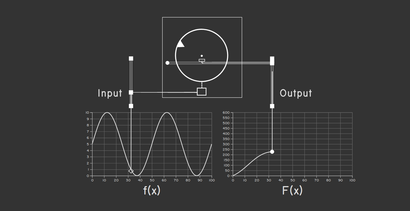A nice screenshot of my visualization, but you should check out the real thing!

So we have a component that can do integration for us, but that alone is not enough to solve a differential equation. To explain the full process to you, I’m going to use an example that Bush offers himself in his 1931 paper, which also happens to be essentially the same example we contemplated in our earlier discussion of differential equations. (This was a happy accident!) Bush introduces the following differential equation to represent the motion of a falling body:

\[\frac{d^2x}{dt^2} = -k\,\frac{dx}{dt} - g\]

This is the same equation we used to model the motion of our tennis ball, only Bush has used \(x\) in place of \(h\) and has added another term that accounts for how air resistance will decelerate the ball. This new term describes the effect of air resistance on the ball in the simplest possible way: The air will slow the ball’s velocity at a rate that is proportional to its velocity (the \(k\) here is some proportionality constant whose value we don’t really care about). So as the ball moves faster, the force of air resistance will be stronger, further decelerating the ball.

To configure a differential analyzer to solve this differential equation, we have to start with what Bush calls the “input table.” The input table is just a piece of graphing paper mounted on a carriage. If we were trying to solve a more complicated equation, the operator of the machine would first plot our input function on the graphing paper and then, once the machine starts running, trace out the function using a pointer connected to the rest of the machine. In this case, though, our input is just the constant \(g\), so we only have to move the pointer to the right value and then leave it there.

What about the other variables \(x\) and \(t\)? The \(x\) variable is our output as it represents the height of the ball. It will be plotted on graphing paper placed on the output table, which is similar to the input table only the pointer is a pen and is driven by the machine. The \(t\) variable should do nothing more than advance at a steady rate. (In our Python simulation of the tennis ball problem as posed earlier, we just incremented \(t\) in a loop.) So the \(t\) variable comes from the differential analyzer’s motor, which kicks off the whole process by rotating the rod connected to it at a constant speed.

Bush has a helpful diagram documenting all of this that I will show you in a second, but first we need to make one more tweak to our differential equation that will make the diagram easier to understand. We can integrate both sides of our equation once, yielding the following:

\[\frac{dx}{dt} = - \int \left(k\,\frac{dx}{dt} + g\right)\,dt\]

The terms in this equation map better to values represented by the rotation of various parts of the machine while it runs. Okay, here’s that diagram:

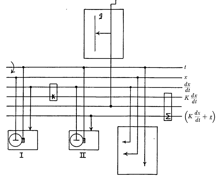The differential analyzer configured to solve the problem of a falling body in one dimension.

The input table is at the top of the diagram. The output table is at the bottom-right. The output table here is set up to graph both \(x\) and \(\frac{dx}{dt}\), i.e. height and velocity. The integrators appear at the bottom-left; since this is a second-order differential equation, we need two. The motor drives the very top rod labeled \(t\). (Interestingly, Bush referred to these horizontal rods as “buses.”)

That leaves two components unexplained. The box with the little \(k\) in it is a multiplier respresnting our proportionality constant \(k\). It takes the rotation of the rod labeled \(\frac{dx}{dt}\) and scales it up or down using a gear ratio. The box with the \(\sum\) symbol is an adder. It uses a clever arrangement of gears to add the rotations of two rods together to drive a third rod. We need it since our equation involves the sum of two terms. These extra components available in the differential analyzer ensure that the machine can flexibly simulate equations with all kinds of terms and coefficients.

I find it helpful to reason in ultra-slow motion about the cascade of cause and effect that plays out as soon as the motor starts running. The motor immediately begins to rotate the rod labeled \(t\) at a constant speed. Thus, we have our notion of time. This rod does three things, illustrated by the three vertical rods connected to it: it drives the rotation of the discs in both integrators and also advances the carriage of the output table so that the output pen begins to draw.

Now if the integrators were set up so that their wheels are centered, then the rotation of rod \(t\) would cause no other rods to rotate. The integrator discs would spin but the wheels, centered as they are, would not be driven. The output chart would just show a flat line. This happens because we have not accounted for the initial conditions of the problem. In our earlier Python simulation, we needed to know the initial velocity of the ball, which we would have represented there as a constant variable or as a parameter of our Python function. Here, we account for the initial velocity and acceleration by displacing the integrator discs by the appropriate amount before the machine begins to run.

Once we’ve done that, the rotation of rod \(t\) propagates through the whole system. Physically, a lot of things start rotating at the same time, but we can think of the rotation going first to integrator II, which combines it with the acceleration expression calculated based on \(g\) and then integrates it to get the result \(\frac{dx}{dt}\). This represents the velocity of the ball. The velocity is in turn used as input to integrator I, whose disc is displaced so that the output wheel rotates at the rate \(\frac{dx}{dt}\). The output from integrator I is our final output \(x\), which gets routed directly to the output table.

One confusing thing I’ve glossed over is that there is a cycle in the machine: Integrator II takes as an input the rotation of the rod labeled \((k\,\frac{dx}{dt} + g)\), but that rod’s rotation is determined in part by the output from integrator II itself. This might make you feel queasy, but there is no physical issue here—everything is rotating at once. If anything, we should not be surprised to see cycles like this, since differential equations often describe rates of change in a function as a function of the function itself. (In this example, the acceleration, which is the rate of change of velocity, depends on the velocity.)

With everything correctly configured, the output we get is a nice graph, charting both the position and velocity of our ball over time. This graph is on paper. To our modern digital sensibilities, that might seem absurd. What can you do with a paper graph? While it’s true that the differential analyzer is not so magical that it can write out a neat mathematical expression for the solution to our problem, it’s worth remembering that neat solutions to many differential equations are not possible anyway. The paper graph that the machine does write out contains exactly the same information that could be output by our earlier Python simulation of a falling ball: where the ball is at any given time. It can be used to answer any practical question you might have about the problem.

The differential analyzer is a preposterously cool machine. It is complicated, but it fundamentally involves nothing more than rotating rods and gears. You don’t have to be an electrical engineer or know how to fabricate a microchip to understand all the physical processes involved. And yet the machine does calculus! It solves differential equations that you never could on your own. The differential analyzer demonstrates that the key material required for the construction of a useful computing machine is not silicon but human ingenuity.

Murdering People

Human ingenuity can serve purposes both good and bad. As I have mentioned, the highest-profile use of differential analyzers historically was to calculate artillery range tables for the US Army. To the extent that the Second World War was the “Good Fight,” this was probably for the best. But there is also no getting past the fact that differential analyzers helped to make very large guns better at killing lots of people. And kill lots of people they did—if Wikipedia is to be believed, more soldiers were killed by artillery than small arms fire during the Second World War.

I will get back to the moralizing in a minute, but just a quick detour here to explain why calculating range tables was hard and how differential analyzers helped, because it’s nice to see how differential analyzers were applied to a real problem. A range table tells the artilleryman operating a gun how high to elevate the barrel to reach a certain range. One way to produce a range table might be just to fire that particular kind of gun at different angles of elevation many times and record the results. This was done at proving grounds like the Aberdeen Proving Ground in Maryland. But producing range tables solely through empirical observation like this is expensive and time-consuming. There is also no way to account for other factors like the weather or for different weights of shell without combinatorially increasing the necessary number of firings to something unmanageable. So using a mathematical theory that can fill in a complete range table based on a smaller number of observed firings is a better approach.

I don’t want to get too deep into how these mathematical theories work, because the math is complicated and I don’t really understand it. But as you might imagine, the physics that governs the motion of an artillery shell in flight is not that different from the physics that governs the motion of a tennis ball thrown upward. The need for accuracy means that the differential equations employed have to depart from the idealized forms we’ve been using and quickly get gnarly. Even the earliest attempts to formulate a rigorous ballistic theory involve equations that account for, among other factors, the weight, diameter, and shape of the projectile, the prevailing wind, the altitude, the atmospheric density, and the rotation of the earth1.

So the equations are complicated, but they are still differential equations that a differential analyzer can solve numerically in the way that we have already seen. Differential analyzers were put to work solving ballistics equations at the Aberdeen Proving Ground in 1935, where they dramatically sped up the process of calculating range tables.2 Nevertheless, during the Second World War, the demand for range tables grew so quickly that the US Army could not calculate them fast enough to accompany all the weaponry being shipped to Europe. This eventually led the Army to fund the ENIAC project at the University of Pennsylvania, which, depending on your definitions, produced the world’s first digital computer. ENIAC could, through rewiring, run any program, but it was constructed primarily to perform range table calculations many times faster than could be done with a differential analyzer.

Given that the range table problem drove much of the early history of computing even apart from the differential analyzer, perhaps it’s unfair to single out the differential analyzer for moral hand-wringing. The differential analyzer isn’t uniquely compromised by its military applications—the entire field of computing, during the Second World War and well afterward, advanced because of the endless funding being thrown at it by the United States military.

Anyway, I think the more interesting legacy of the differential analyzer is what it teaches us about the nature of computing. I am surprised that the differential analyzer can accomplish as much as it can; my guess is that you are too. It is easy to fall into the trap of thinking of computing as the realm of what can be realized with very fast digital circuits. In truth, computing is a more abstract process than that, and electronic, digital circuits are just what we typically use to get it done. In his paper about the differential analyzer, Vannevar Bush suggests that his invention is just a small contribution to “the far-reaching project of utilizing complex mechanical interrelationships as substitutes for intricate processes of reasoning.” That puts it nicely.

If you enjoyed this post, more like it come out every four weeks! Follow @TwoBitHistory on Twitter or subscribe to the RSS feed to make sure you know when a new post is out.

Previously on TwoBitHistory…

Do you worry that your children are "BBS-ing"? Do you have a neighbor who talks too much about his "door games"?

In this VICE News special report, we take you into the seedy underworld of bulletin board systems: https://t.co/hBrKGU2rfB

— TwoBitHistory (@TwoBitHistory) February 2, 2020

]]>Bulletin Board Systems: The VICE Exposé2020-02-02T00:00:00+00:002020-02-02T00:00:00+00:00https://twobithistory.org/2020/02/02/bbsBy now, you have almost certainly heard of the dark web. On sites unlisted by any search engine, in forums that cannot be accessed without special passwords or protocols, criminals and terrorists meet to discuss conspiracy theories and trade child pornography.

We here at VICE headquarters have reported before on the dark web’s [“hurtcore”
communities](https://www.vice.com/en_us/article/mbxqqy/a-journey-into-the-worst-corners-of-the-dark-web), its [human trafficking
markets](https://www.vice.com/en_us/article/vvbazy/my-brief-encounter-with-a-dark-web-human-trafficking-site), its [rent-a-hitman
websites](https://www.vice.com/en_us/article/3d434v/a-fake-dark-web-hitman-site-is-linked-to-a-real-murder). We have explored [the challenges the dark web presents to
regulators](https://www.vice.com/en_us/article/ezv85m/problem-the-government-still-doesnt-understand-the-dark-web), the rise of [dark web revenge
porn](https://www.vice.com/en_us/article/53988z/revenge-porn-returns-to-the-dark-web), and the frightening size of [the dark web gun
trade](https://www.vice.com/en_us/article/j5qnbg/dark-web-gun-trade-study-rand). We have kept you informed about that one dark web forum where you can make like Walter White and [learn how to manufacture your own
drugs](https://www.vice.com/en_ca/article/wj374q/inside-the-dark-web-forum-that-tells-you-how-to-make-drugs), and also about—thanks to our foreign correspondent— [the Chinese dark
web](https://www.vice.com/en_us/article/4x38ed/the-chinese-deep-web-takes-a-darker-turn). We have even attempted to [catalog every single location on the dark
web](https://www.vice.com/en_us/article/vv57n8/here-is-a-list-of-every-single-possible-dark-web-site). Our coverage of the dark web has been nothing if not comprehensive.

But I wanted to go deeper.

We know that below the surface web is the deep web, and below the deep web is the dark web. It stands to reason that below the dark web there should be a deeper, darker web.

A month ago, I set out to find it. Unsure where to start, I made a post on Reddit, a website frequented primarily by cosplayers and computer enthusiasts. I asked for a guide, a Styx ferryman to bear me across to the mythical underworld I sought to visit.

Only minutes after I made my post, I received a private message. “If you want to see it, I’ll take you there,” wrote Reddit user FingerMyKumquat. “But I’ll warn you just once—it’s not pretty to see.”

Getting Access

This would not be like visiting Amazon to shop for toilet paper. I could not just enter an address into the address bar of my browser and hit go. In fact, as my Charon informed me, where we were going, there are no addresses. At least, no web addresses.

But where exactly were we going? The answer: Back in time. The deepest layer of the internet is also the oldest. Down at this deepest layer exists a secret society of “bulletin board systems,” a network of underground meetinghouses that in some cases have been in continuous operation since the 1980s—since before Facebook, before Google, before even stupidvideos.com.

To begin, I needed to download software that could handle the ancient protocols used to connect to the meetinghouses. I was told that bulletin board systems today use an obsolete military protocol called Telnet. Once upon a time, though, they operated over the phone lines. To connect to a system back then you had to dial its phone number.

The software I needed was called SyncTerm. It was not available on the App Store. In order to install it, I had to compile it. This is a major barrier to entry, I am told, even to veteran computer programmers.

When I had finally installed SyncTerm, my guide said he needed to populate my directory. I asked what that was a euphemism for, but was told it was not a euphemism. Down this far, there are no search engines, so you can only visit the bulletin board systems you know how to contact. My directory was the list of bulletin board systems I would be able to contact. My guide set me up with just seven, which he said would be more than enough.

More than enough for what, I wondered. Was I really prepared to go deeper than the dark web? Was I ready to look through this window into the black abyss of the human soul?

The vivid blue interface of SyncTerm. My directory of BBSes on the left.

Heatwave

I decided first to visit the bulletin board system called “Heatwave,” which I imagined must be a hangout for global warming survivalists. I “dialed” in. The next thing I knew, I was being asked if I wanted to create a user account. I had to be careful to pick an alias that would be inconspicuous in this sub-basement of the internet. I considered “DonPablo,” and “z3r0day,” but finally chose “ripper”—a name I could remember because it is also the name of my great-aunt Meredith’s Shih Tzu. I was then asked where I was dialing from; I decided “xxx” was the right amount of enigmatic.

And then—I was in. Curtains of fire rolled down my screen and dispersed, revealing the main menu of the Heatwave bulletin board system.

The main menu of the Heatwave BBS.

I had been told that even in the glory days of bulletin board systems, before the rise of the world wide web, a large system would only have several hundred users or so. Many systems were more exclusive, and most served only users in a single telephone area code. But how many users dialed the “Heatwave” today? There was a main menu option that read “(L)ast Few Callers,” so I hit “L” on my keyboard.

My screen slowly filled with a large table, listing all of the system’s “callers” over the last few days. Who were these shadowy outcasts, these expert hackers, these denizens of the digital demimonde? My eyes scanned down the list, and what I saw at first confused me: There was a “Dan,” calling from St. Louis, MO. There was also a “Greg Miller,” calling from Portland, OR. Another caller claimed he was “George” calling from Campellsburg, KY. Most of the entries were like that.

It was a joke, of course. A meme, a troll. It was normcore fashion in noms de guerre. These were thrill-seeking Palo Alto adolescents on Adderall making fun of the surface web. They weren’t fooling me.

I wanted to know what they talked about with each other. What cryptic colloquies took place here, so far from public scrutiny? My index finger, with ever so slight a tremble, hit “M” for “(M)essage Areas.”

Here, I was presented with a choice. I could enter the area reserved for discussions about “T-99 and Geneve,” which I did not dare do, not knowing what that could possibly mean. I could also enter the area for discussions about “Other,” which seemed like a safe place to start.

The system showed me message after message. There was advice about how to correctly operate a leaf-blower, as well as a protracted debate about the depth of the Strait of Hormuz relative to the draft of an aircraft carrier. I assumed the real messages were further on, and indeed I soon spotted what I was looking for. The user “Kevin” was complaining to other users about the side effects of a drug called Remicade. This was not a drug I had heard of before. Was it some powerful new synthetic stimulant? A cocktail of other recreational drugs? Was it something I could bring with me to impress people at the next VICE holiday party?

I googled it. Remicade is used to treat rheumatoid arthritis and Crohn’s disease.

In reply to the original message, there was some further discussion about high resting heart rates and mechanical heart valves. I decided that I had gotten lost and needed to contact FingerMyKumquat. “Finger,” I messaged him, “What is this shit I’m looking at here? I want the real stuff. I want blackmail and beheadings. Show me the scum of the earth!”

“Perhaps you’re ready for the SpookNet,” he wrote back.

SpookNet

Each bulletin board system is an island in the television-static ocean of the digital world. Each system’s callers are lonely sailors come into port after many a month plying the seas.

But the bulletin board systems are not entirely disconnected. Faint phosphorescent filaments stretch between the islands, links in the special-purpose networks that were constructed—before the widespread availability of the internet—to propagate messages from one system to another.

One such network is the SpookNet. Not every bulletin board system is connected to the SpookNet. To get on, I first had to dial “Reality Check.”

The Reality Check BBS.

Once I was in, I navigated my way past the main menu and through the SpookNet gateway. What I saw then was like a catalog index for everything stored in that secret Pentagon warehouse from the end of the X-Files pilot. There were message boards dedicated to UFOs, to cryptography, to paranormal studies, and to “End Times and the Last Days.” There was a board for discussing “Truth, Polygraphs, and Serums,” and another for discussing “Silencers of Information.” Here, surely, I would find something worth writing about in an article for VICE.

I browsed and I browsed. I learned about which UFO documentaries are worth watching on Netflix. I learned that “paper mill” is a derogatory term used in the intelligence community (IC) to describe individuals known for constantly trying to sell “explosive” or “sensitive” documents—as in the sentence, offered as an example by one SpookNet user, “Damn, here comes that paper mill Juan again.” I learned that there was an effort afoot to get two-factor authentication working for bulletin board systems.

“These are just a bunch of normal losers,” I finally messaged my guide. “Mostly they complain about anti-vaxxers and verses from the Quran. This is just Reddit!”

“Huh,” he replied. “When you said ‘scum of the earth,’ did you mean something else?”

I had one last idea. In their heyday, bulletin board systems were infamous for being where everyone went to download illegal, cracked computer software. An entire subculture evolved, with gangs of software pirates competing to be the first to crack a new release. The first gang to crack the new software would post their “warez” for download along with a custom piece of artwork made using lo-fi ANSI graphics, which served to identify the crack as their own.

I wondered if there were any old warez to be found on the Reality Check BBS. I backed out of the SpookNet gateway and keyed my way to the downloads area. There were many files on offer there, but one in particular caught my attention: a 5.3 megabyte file just called “GREY.”

I downloaded it. It was a complete PDF copy of E. L. James’ 50 Shades of Grey.

If you enjoyed this post, more like it come out every four weeks! Follow @TwoBitHistory on Twitter or subscribe to the RSS feed to make sure you know when a new post is out.

Previously on TwoBitHistory…

I first heard about the FOAF (Friend of a Friend) standard back when I wrote my post about the Semantic Web. I thought it was a really interesting take on social networking and I've wanted to write about it since. Finally got around to it! https://t.co/VNwT8wgH8j

— TwoBitHistory (@TwoBitHistory) January 5, 2020

]]>Friend of a Friend: The Facebook That Could Have Been2020-01-05T00:00:00+00:002020-01-05T00:00:00+00:00https://twobithistory.org/2020/01/05/foaf

I express my network in a FOAF file, and that is the start of the revolution. —Tim Berners-Lee (2007)

The FOAF standard, or Friend of a Friend standard, is a now largely defunct/ignored/superseded1 web standard dating from the early 2000s that hints at what social networking might have looked like had Facebook not conquered the world. Before we talk about FOAF though, I want to talk about the New York City Subway.

The New York City Subway is controlled by a single entity, the Metropolitan Transportation Agency, better known as the MTA. The MTA has a monopoly on subway travel in New York City. There is no legal way to travel in New York City by subway without purchasing a ticket from the MTA. The MTA has no competitors, at least not in the “subway space.”

This wasn’t always true. Surprisingly, the subway system was once run by two corporations that competed with each other. The Inter-borough Rapid Transit Company (IRT) operated lines that ran mostly through Manhattan, while the Brooklyn-Manhattan Transit Corporation (BMT) operated lines in Brooklyn, some of which extended into Manhattan also. In 1932, the City opened its own service called the Independent Subway System to compete with the IRT and BMT, and so for a while there were three different organizations running subway lines in New York City.

One imagines that this was not an effective way to run a subway. It was not. Constructing interchanges between the various systems was challenging because the IRT and BMT used trains of different widths. Interchange stations also had to have at least two different fare-collection areas since passengers switching trains would have to pay multiple operators. The City eventually took over the IRT and BMT in 1940, bringing the whole system together under one operator, but some of the inefficiencies that the original division entailed are still problems today: Trains designed to run along lines inherited from the BMT (e.g. the A, C, or E) cannot run along lines inherited from the IRT (e.g. the 1, 2, or 3) because the IRT tunnels are too narrow. As a result, the MTA has to maintain two different fleets of mutually incompatible subway cars, presumably at significant additional expense relative to other subway systems in the world that only have to deal with a single tunnel width.

This legacy of the competition between the IRT and BMT suggests that subway systems naturally tend toward monopoly. It just makes more sense for there to be a single operator than for there to be competing operators. Average passengers are amply compensated for the loss of choice by never having to worry about whether they brought their IRT MetroCard today but forgot their BMT MetroCard at home.

Okay, so what does the Subway have to do with social networking? Well, I have wondered for a while now whether Facebook has, like the MTA, a natural monopoly. Facebook does seem to have a monopoly, whether natural or unnatural—not over social media per se (I spend much more time on Twitter), but over my internet social connections with real people I know. It has a monopoly over, as they call it, my digitized “social graph”; I would quit Facebook tomorrow if I didn’t worry that by doing so I might lose many of those connections. I get angry about this power that Facebook has over me. I get angry in a way that I do not get angry about the MTA, even though the Subway is, metaphorically and literally, a sprawling trash fire. And I suppose I get angry because at root I believe that Facebook’s monopoly, unlike the MTA’s, is not a natural one.

What this must mean is that I think Facebook owns all of our social data now because they happened to get there first and then dig a big moat around themselves, not because a world with competing Facebook-like platforms is inefficient or impossible. Is that true, though? There are some good reasons to think it isn’t: Did Facebook simply get there first, or did they instead just do social networking better than everyone else? Isn’t the fact that there is only one Facebook actually convenient if you are trying to figure out how to contact an old friend? In a world of competing Facebooks, what would it mean if you and your boyfriend are now Facebook official, but he still hasn’t gotten around to updating his relationship status on VisageBook, which still says he is in a relationship with his college ex? Which site will people trust? Also, if there were multiple sites, wouldn’t everyone spend a lot more time filling out web forms?

In the last few years, as the disadvantages of centralized social networks have dramatically made themselves apparent, many people have attempted to create decentralized alternatives. These alternatives are based on open standards that could potentially support an ecosystem of inter-operating social networks (see e.g. the Fediverse). But none of these alternatives has yet supplanted a dominant social network. One obvious explanation for why this hasn’t happened is the power of network effects: With everyone already on Facebook, any one person thinking of leaving faces a high cost for doing so. Some might say this proves that social networks are natural monopolies and stop there; I would say that Facebook, Twitter, et al. chose to be walled gardens, and given that people have envisioned and even built social networks that inter-operate, the network effects that closed platforms enjoy tell us little about the inherent nature of social networks.

So the real question, in my mind, is: Do platforms like Facebook continue to dominate merely because of their network effects, or is having a single dominant social network more efficient in the same way that having a single operator for a subway system is more efficient?

Which finally brings me back to FOAF. Much of the world seems to have forgotten about the FOAF standard, but FOAF was an attempt to build a decentralized and open social network before anyone had even heard of Facebook. If any decentralized social network ever had a chance of occupying the redoubt that Facebook now occupies before Facebook got there, it was FOAF. Given that a large fraction of humanity now has a Facebook account, and given that relatively few people know about FOAF, should we conclude that social networking, like subway travel, really does lend itself to centralization and natural monopoly? Or does the FOAF project demonstrate that decentralized social networking was a feasible alternative that never became popular for other reasons?

The Future from the Early Aughts

The FOAF project, begun in 2000, set out to create a universal standard for describing people and the relationships between them. That might strike you as a wildly ambitious goal today, but aspirations like that were par for the course in the late 1990s and early 2000s. The web (as people still called it then) had just trounced closed systems like America Online and Prodigy. It could only have been natural to assume that further innovation in computing would involve the open, standards-based approach embodied by the web.

Many people believed that the next big thing was for the web to evolve into something called the Semantic Web. I have written about what exactly the Semantic Web was supposed to be and how it was supposed to work before, so I won’t go into detail here. But I will sketch the basic vision motivating the people who worked on Semantic Web technologies, because the FOAF standard was an application of that vision to social networking.

There is an essay called [“How Google beat Amazon and Ebay to the Semantic
Web”](https://www.ftrain.com/google_takes_all) that captures the lofty dream of the Semantic Web well. It was written by Paul Ford in 2002. The essay imagines a future (as imminent as 2009) in which Google, by embracing the Semantic Web, has replaced Amazon and eBay as the dominant e-commerce platform. In this future, you can search for something you want to purchase—perhaps a second-hand Martin guitar—by entering buy:martin guitar into Google. Google then shows you all the people near your zipcode selling Martin guitars. Google knows about these people and their guitars because Google can read RDF, a markup language and core Semantic Web technology focused on expressing relationships. Regular people can embed RDF on their web pages to advertise (among many other things) the items they have to sell. Ford predicts that as the number of people searching for and advertising products this way grows, Amazon and eBay will lose their near-monopolies over, respectively, first-hand and second-hand e-commerce. Nobody will want to search a single centralized database for something to buy when they could instead search the whole web. Even Google, Ford writes, will eventually lose its advantage, because in theory anyone could crawl the web reading RDF and offer a search feature similar to Google’s. At the very least, if Google wanted to make money from its Semantic Web marketplace by charging a percentage of each transaction, that percentage would probably by forced down over time by competitors offering a more attractive deal.

Ford’s imagined future was an application of RDF, or the Resource Description Framework, to e-commerce, but the exciting thing about RDF was that hypothetically it could be used for anything. The RDF standard, along with a constellation of related standards, once widely adopted, was supposed to blow open database-backed software services on the internet the same way HTML had blown open document publishing on the internet.

One arena that RDF and other Semantic Web technologies seemed poised to takeover immediately was social networking. The FOAF project, known originally as “RDF Web Ring” before being renamed, was the Semantic Web effort offshoot that sought to accomplish this. FOAF was so promising in its infancy that some people thought it would inevitably make all other social networking sites obsolete. A 2004 Guardian article about the project introduced FOAF this way:

In the beginning, way back in 1996, it was SixDegrees. Last year, it was Friendster. Last week, it was Orkut. Next week, it could be Flickr. All these websites, and dozens more, are designed to build networks of friends, and they are currently at the forefront of the trendiest internet development: social networking. But unless they can start to offer more substantial benefits, it is hard to see them all surviving, once the Friend Of A Friend (FOAF) standard becomes a normal part of life on the net.2

The article goes on to complain that the biggest problem with social networking is that there are too many social networking sites. Something is needed that can connect all of the different networks together. FOAF is the solution, and it will revolutionize social networking as a result.

FOAF, according to the article, would tie the different networks together by doing three key things:

• It would establish a machine-readable format for social data that could be read by any social networking site, saving users from having to enter this information over and over again
• It would allow “personal information management programs,” i.e. your “Contacts” application, to generate a file in this machine-readable format that you could feed to social networking sites
• It would further allow this machine-readable format to be hosted on personal homepages and read remotely by social networking sites, meaning that you would be able to keep your various profiles up-to-date by just pushing changes to your own homepage

It is hard to believe today, but the problem in 2004, at least for savvy webizens and technology columnists aware of all the latest sites, was not the lack of alternative social networks but instead the proliferation of them. Given that problem—so alien to us now—one can see why it made sense to pursue a single standard that promised to make the proliferation of networks less of a burden.

The FOAF Spec

According to the description currently given on the FOAF project’s website, FOAF is “a computer language defining a dictionary of people-related terms that can be used in structured data.” Back in 2000, in a document they wrote to explain the project’s goals, Dan Brickley and Libby Miller, FOAF’s creators, offered a different description that suggests more about the technology’s ultimate purpose—they introduced FOAF as a tool that would allow computers to read the personal information you put on your homepage the same way that other humans do.3 FOAF would “help the web do the sorts of things that are currently the proprietary offering of centralised services.”4 By defining a standard vocabulary for people and the relationships between them, FOAF would allow you to ask the web questions such as, “Find me today’s web recommendations made by people who work for Medical organizations,” or “Find me recent publications by people I’ve co-authored documents with.”

Since FOAF is a standardized vocabulary, the most important output of the FOAF project was the FOAF specification. The FOAF specification defines a small collection of RDF classes and RDF properties. (I’m not going to explain RDF here, but again see my post about the Semantic Web if you want to know more.) The RDF classes defined by the FOAF specification represent subjects you might want to describe, such as people (the Person class) and organizations (the Organization class). The RDF properties defined by the FOAF specification represent logical statements you might make about the different subjects. A person could have, for example, a first name (the givenName property), a last name (the familyName property), perhaps even a personality type (the myersBriggs property), and be near another person or location (the based_near property). The idea was that these classes and properties would be sufficient to represent the kind of the things people say about themselves and their friends on their personal homepage.

The FOAF specification gives the following as an example of a well-formed FOAF document. This example uses XML, though an equivalent document could be written using JSON or a number of other formats:

<foaf:Person rdf:about="#danbri" xmlns:foaf="http://xmlns.com/foaf/0.1/">
  <foaf:name>Dan Brickley</foaf:name>
  <foaf:homepage rdf:resource="http://danbri.org/" />
  <foaf:openid rdf:resource="http://danbri.org/" />
  <foaf:img rdf:resource="/images/me.jpg" />
</foaf:Person>

This FOAF document describes a person named “Dan Brickley” (one of the specification’s authors) that has a homepage at http://danbri.org, something called an “open ID,” and a picture available at /images/me.jpg, presumably relative to the base address of Brickley’s homepage. The FOAF-specific terms are prefixed by foaf:, indicating that they are part of the FOAF namespace, while the more general RDF terms are prefixed by rdf:.

Just to persuade you that FOAF isn’t tied to XML, here is a similar FOAF example from Wikipedia, expressed using a format called JSON-LD5:

{
  "@context": {
    "name": "http://xmlns.com/foaf/0.1/name",
    "homepage": {
      "@id": "http://xmlns.com/foaf/0.1/workplaceHomepage",
      "@type": "@id"
    },
    "Person": "http://xmlns.com/foaf/0.1/Person"
  },
  "@id": "https://me.example.com",
  "@type": "Person",
  "name": "John Smith",
  "homepage": "https://www.example.com/"
}

This FOAF document describes a person named John Smith with a homepage at www.example.com.

Perhaps the best way to get a feel for how FOAF works is to play around with FOAF-a-matic, a web tool for generating FOAF documents. It allows you to enter information about yourself using a web form, then uses that information to create the FOAF document (in XML) that represents you. FOAF-a-matic demonstrates how FOAF could have been used to save everyone from having to enter their social information into a web form ever again—if every social networking site could read FOAF, all you’d need to do to sign up for a new site is point the site to the FOAF document that FOAF-a-matic generated for you.

Here is a slightly more complicated FOAF example, representing me, that I created using FOAF-a-matic:

<rdf:RDF
      xmlns:rdf="http://www.w3.org/1999/02/22-rdf-syntax-ns#"
      xmlns:rdfs="http://www.w3.org/2000/01/rdf-schema#"
      xmlns:foaf="http://xmlns.com/foaf/0.1/"
      xmlns:admin="http://webns.net/mvcb/">
  <foaf:PersonalProfileDocument rdf:about="">
    <foaf:maker rdf:resource="#me"/>
    <foaf:primaryTopic rdf:resource="#me"/>
    <admin:generatorAgent rdf:resource="http://www.ldodds.com/foaf/foaf-a-matic"/>
    <admin:errorReportsTo rdf:resource="mailto:[email protected]"/>
  </foaf:PersonalProfileDocument>
  <foaf:Person rdf:ID="me">
    <foaf:name>Sinclair Target</foaf:name>
    <foaf:givenname>Sinclair</foaf:givenname>
    <foaf:family_name>Target</foaf:family_name>
    <foaf:mbox rdf:resource="mailto:[email protected]"/>
    <foaf:homepage rdf:resource="sinclairtarget.com"/>
    <foaf:knows>
      <foaf:Person>
        <foaf:name>John Smith</foaf:name>
        <foaf:mbox rdf:resource="mailto:[email protected]"/>
        <rdfs:seeAlso rdf:resource="www.example.com/foaf.rdf"/>
      </foaf:Person>
    </foaf:knows>
  </foaf:Person>
</rdf:RDF>

This example has quite a lot of preamble setting up the various XML namespaces used by the document. There is also a section containing data about the tool that was used to generate the document, largely so that, it seems, people know whom to email with complaints. The foaf:Person element describing me tells you my name, email address, and homepage. There is also a nested foaf:knows element telling you that I am friends with John Smith.

This example illustrates another important feature of FOAF documents: They can link to each other. If you remember from the previous example, my friend John Smith has a homepage at www.example.com. In this example, where I list John Smith as a foaf:person with whom I have a foaf:knows relationship, I also provide a rdfs:seeAlso element that points to John Smith’s FOAF document hosted on his homepage. Because I have provided this link, any program reading my FOAF document could find out more about John Smith by following the link and reading his FOAF document. In the FOAF document we have for John Smith above, John did not provide any information about his friends (including me, meaning, tragically, that our friendship is unidirectional). But if he had, then the program reading my document could find out not only about me but also about John, his friends, their friends, and so on, until the program has crawled the whole social graph that John and I inhabit.

This functionality will seem familiar to anyone that has used Facebook, which is to say that this functionality will seem familiar to you. There is no foaf:wall property or foaf:poke property to replicate Facebook’s feature set exactly. Obviously, there is also no slick blue user interface that everyone can use to visualize their FOAF social network; FOAF is just a vocabulary. But Facebook’s core feature—the feature that I have argued is key to Facebook’s monopoly power over, at the very least, myself—is here provided in a distributed way. FOAF allows a group of friends to represent their real-life social graph digitally by hosting FOAF documents on their own homepages. It allows them to do this without surrendering control of their data to a centralized database in the sky run by a billionaire android-man who spends much of his time apologizing before congressional committees.

FOAF on Ice

If you visit the current FOAF project homepage, you will notice that, in the top right corner, there is an image of the character Fry from the TV series Futurama, stuck inside some sort of stasis chamber. This is a still from the pilot episode of Futurama, in which Fry gets frozen in a cryogenic tank in 1999 only to awake a millennium later in 2999. Brickley, whom I messaged briefly on Twitter, told me that he put that image there as a way communicating that the FOAF project is currently “in stasis,” though he hopes that there will be a future opportunity to resuscitate the project along with its early 2000s optimism about how the web should work.

FOAF never revolutionized social networking the way that the 2004 Guardian article about it expected it would. Some social networking sites decided to support the standard: LiveJournal and MyOpera are examples.6 FOAF even played a role in Howard Dean’s presidential campaign in 2004—a group of bloggers and programmers got together to create a network of websites they called “DeanSpace” to promote the campaign, and these sites used FOAF to keep track of supporters and volunteers.7 But today FOAF is known primarily for being one of the more widely used vocabularies of RDF, itself a niche standard on the modern web. If FOAF is part of your experience of the web today at all, then it is as an ancestor to the technology that powers Google’s “knowledge panels” (the little sidebars that tell you the basics about a person or a thing if you searched for something simple). Google uses vocabularies published by the schema.org project—the modern heir to the Semantic Web effort—to populate its knowledge panels.8 The schema.org vocabulary for describing people seems to be somewhat inspired by FOAF and serves many of the same purposes.

So why didn’t FOAF succeed? Why do we all use Facebook now instead? Let’s ignore that FOAF is a simple standard with nowhere near as many features as Facebook—that’s true today, clearly, but if FOAF had enjoyed more momentum it’s possible that applications could have been built on top of it to deliver a Facebook-like experience. The interesting question is: Why didn’t this nascent form of distributed social networking catch fire when Facebook was not yet around to compete with it?

There probably is no single answer to that question, but if I had to pick one, I think the biggest issue is that FOAF only makes sense on a web where everyone has a personal website. In the late 1990s and early 2000s, it might have been easy to assume the web would eventually look like this, especially since so many of the web’s early adopters were, as far as I can tell, prolific bloggers or politically engaged technologists excited to have a platform. But the reality is that regular people don’t want to have to learn how to host a website. FOAF allows you to control your own social information and broadcast it to social networks instead of filling out endless web forms, which sounds pretty great if you already have somewhere to host that information. But most people in practice found it easier to just fill out the web form and sign up for Facebook than to figure out how to buy a domain and host some XML.

What does this mean for my original question about whether or not Facebook’s monopoly is a natural one? I think I have to concede that the FOAF example is evidence that social networking does naturally lend itself to monopoly.

That people did not want to host their own data isn’t especially meaningful itself—modern distributed social networks like Mastodon have solved that problem by letting regular users host their profiles on nodes set up by more savvy users. It is a sign, however, of just how much people hate complexity. This is bad news for decentralized social networks, because they are inherently more complex under the hood than centralized networks in a way that is often impossible to hide from users.

Consider FOAF: If I were to write an application that read FOAF data from personal websites, what would I do if Sally’s FOAF document mentions a John Smith with a homepage at example.com, and Sue’s FOAF document mentions a John Smith with a homepage at example.net? Are we talking about a single John Smith with two websites or two entirely different John Smiths? What if the both FOAF documents list John Smith’s email as [email protected]? This issue of identity was an acute one for FOAF. In a 2003 email, Brickley wrote that because there does not exist and probably should not exist a “planet-wide system for identifying people,” the approach taken by FOAF is “pluralistic.”9 Some properties of FOAF people, such as email addresses and homepage addresses, are special in that their values are globally unique. So these different properties can be used to merge (or, as Libby Miller called it, “smoosh”) FOAF documents about people together. But none of these special properties are privileged above the others, so it’s not obvious how to handle our John Smith case. Do we trust the homepages and conclude we have two different people? Or do we trust the email addresses and conclude we have a single person? Could I really write an application capable of resolving this conflict without involving (and inconveniencing) the user?

Facebook, with its single database and lack of political qualms, could create a “planet-wide system for identifying people” and so just gave every person a unique Facebook ID. Problem solved.

Complexity alone might not doom distributed social networks if people cared about being able to own and control their data. But FOAF’s failure to take off demonstrates that people have never valued control very highly. As one blogger has put it, “‘Users want to own their own data’ is an ideology, not a use case.”10 If users do not value control enough to stomach additional complexity, and if centralized systems are more simple than distributed ones—and if, further, centralized systems tend to be closed and thus the successful ones enjoy powerful network effects—then social networks are indeed natural monopolies.

That said, I think there is still a distinction to be drawn between the subway system case and the social networking case. I am comfortable with the MTA’s monopoly on subway travel because I expect subway systems to be natural monopolies for a long time to come. If there is going to be only one operator of the New York City Subway, then it ought to be the government, which is at least nominally more accountable than a private company with no competitors. But I do not expect social networks to stay natural monopolies. The Subway is carved in granite; the digital world is writ in water. Distributed social networks may now be more complicated than centralized networks in the same way that carrying two MetroCards is more complicated than carrying one. In the future, though, the web, or even the internet, could change in fundamental ways that make distributed technology much easier to use.

If that happens, perhaps FOAF will be remembered as the first attempt to build the kind of social network that humanity, after a brief experiment with corporate mega-databases, does and always will prefer.

If you enjoyed this post, more like it come out every four weeks! Follow @TwoBitHistory on Twitter or subscribe to the RSS feed to make sure you know when a new post is out.

Previously on TwoBitHistory…

I know it's been too long since my last post, but my new one is here! I wrote almost 5000 words on John Carmack, Doom, and the history of the binary space partitioning tree. https://t.co/SVunDZ0hZ1

— TwoBitHistory (@TwoBitHistory) November 6, 2019

]]>How Much of a Genius-Level Move Was Using Binary Space Partitioning in Doom?2019-11-06T00:00:00+00:002019-11-06T00:00:00+00:00https://twobithistory.org/2019/11/06/doom-bspIn 1993, id Software released the first-person shooter Doom, which quickly became a phenomenon. The game is now considered one of the most influential games of all time.

A decade after Doom’s release, in 2003, journalist David Kushner published a book about id Software called Masters of Doom, which has since become the canonical account of Doom’s creation. I read Masters of Doom a few years ago and don’t remember much of it now, but there was one story in the book about lead programmer John Carmack that has stuck with me. This is a loose gloss of the story (see below for the full details), but essentially, early in the development of Doom, Carmack realized that the 3D renderer he had written for the game slowed to a crawl when trying to render certain levels. This was unacceptable, because Doom was supposed to be action-packed and frenetic. So Carmack, realizing the problem with his renderer was fundamental enough that he would need to find a better rendering algorithm, started reading research papers. He eventually implemented a technique called “binary space partitioning,” never before used in a video game, that dramatically sped up the Doom engine.

That story about Carmack applying cutting-edge academic research to video games has always impressed me. It is my explanation for why Carmack has become such a legendary figure. He deserves to be known as the archetypal genius video game programmer for all sorts of reasons, but this episode with the academic papers and the binary space partitioning is the justification I think of first.

Obviously, the story is impressive because “binary space partitioning” sounds like it would be a difficult thing to just read about and implement yourself. I’ve long assumed that what Carmack did was a clever intellectual leap, but because I’ve never understood what binary space partitioning is or how novel a technique it was when Carmack decided to use it, I’ve never known for sure. On a spectrum from Homer Simpson to Albert Einstein, how much of a genius-level move was it really for Carmack to add binary space partitioning to Doom?

I’ve also wondered where binary space partitioning first came from and how the idea found its way to Carmack. So this post is about John Carmack and Doom, but it is also about the history of a data structure: the binary space partitioning tree (or BSP tree). It turns out that the BSP tree, rather interestingly, and like so many things in computer science, has its origins in research conducted for the military.

That’s right: E1M1, the first level of Doom, was brought to you by the US Air Force.

The VSD Problem

The BSP tree is a solution to one of the thorniest problems in computer graphics. In order to render a three-dimensional scene, a renderer has to figure out, given a particular viewpoint, what can be seen and what cannot be seen. This is not especially challenging if you have lots of time, but a respectable real-time game engine needs to figure out what can be seen and what cannot be seen at least 30 times a second.

This problem is sometimes called the problem of visible surface determination. Michael Abrash, a programmer who worked with Carmack on Quake (id Software’s follow-up to Doom), wrote about the VSD problem in his famous Graphics Programming Black Book:

I want to talk about what is, in my opinion, the toughest 3-D problem of all: visible surface determination (drawing the proper surface at each pixel), and its close relative, culling (discarding non-visible polygons as quickly as possible, a way of accelerating visible surface determination). In the interests of brevity, I’ll use the abbreviation VSD to mean both visible surface determination and culling from now on.

Why do I think VSD is the toughest 3-D challenge? Although rasterization issues such as texture mapping are fascinating and important, they are tasks of relatively finite scope, and are being moved into hardware as 3-D accelerators appear; also, they only scale with increases in screen resolution, which are relatively modest.

In contrast, VSD is an open-ended problem, and there are dozens of approaches currently in use. Even more significantly, the performance of VSD, done in an unsophisticated fashion, scales directly with scene complexity, which tends to increase as a square or cube function, so this very rapidly becomes the limiting factor in rendering realistic worlds.1

Abrash was writing about the difficulty of the VSD problem in the late ’90s, years after Doom had proved that regular people wanted to be able to play graphically intensive games on their home computers. In the early ’90s, when id Software first began publishing games, the games had to be programmed to run efficiently on computers not designed to run them, computers meant for word processing, spreadsheet applications, and little else. To make this work, especially for the few 3D games that id Software published before Doom, id Software had to be creative. In these games, the design of all the levels was constrained in such a way that the VSD problem was easier to solve.

For example, in Wolfenstein 3D, the game id Software released just prior to Doom, every level is made from walls that are axis-aligned. In other words, in the Wolfenstein universe, you can have north-south walls or west-east walls, but nothing else. Walls can also only be placed at fixed intervals on a grid—all hallways are either one grid square wide, or two grid squares wide, etc., but never 2.5 grid squares wide. Though this meant that the id Software team could only design levels that all looked somewhat the same, it made Carmack’s job of writing a renderer for Wolfenstein much simpler.

The Wolfenstein renderer solved the VSD problem by “marching” rays into the virtual world from the screen. Usually a renderer that uses rays is a “raycasting” renderer—these renderers are often slow, because solving the VSD problem in a raycaster involves finding the first intersection between a ray and something in your world, which in the general case requires lots of number crunching. But in Wolfenstein, because all the walls are aligned with the grid, the only location a ray can possibly intersect a wall is at the grid lines. So all the renderer needs to do is check each of those intersection points. If the renderer starts by checking the intersection point nearest to the player’s viewpoint, then checks the next nearest, and so on, and stops when it encounters the first wall, the VSD problem has been solved in an almost trivial way. A ray is just marched forward from each pixel until it hits something, which works because the marching is so cheap in terms of CPU cycles. And actually, since all walls are the same height, it is only necessary to march a single ray for every column of pixels.

This rendering shortcut made Wolfenstein fast enough to run on underpowered home PCs in the era before dedicated graphics cards. But this approach would not work for Doom, since the id team had decided that their new game would feature novel things like diagonal walls, stairs, and ceilings of different heights. Ray marching was no longer viable, so Carmack wrote a different kind of renderer. Whereas the Wolfenstein renderer, with its ray for every column of pixels, is an “image-first” renderer, the Doom renderer is an “object-first” renderer. This means that rather than iterating through the pixels on screen and figuring out what color they should be, the Doom renderer iterates through the objects in a scene and projects each onto the screen in turn.

In an object-first renderer, one easy way to solve the VSD problem is to use a z-buffer. Each time you project an object onto the screen, for each pixel you want to draw to, you do a check. If the part of the object you want to draw is closer to the player than what was already drawn to the pixel, then you can overwrite what is there. Otherwise you have to leave the pixel as is. This approach is simple, but a z-buffer requires a lot of memory, and the renderer may still expend a lot of CPU cycles projecting level geometry that is never going to be seen by the player.

In the early 1990s, there was an additional drawback to the z-buffer approach: On IBM-compatible PCs, which used a video adapter system called VGA, writing to the output frame buffer was an expensive operation. So time spent drawing pixels that would only get overwritten later tanked the performance of your renderer.

Since writing to the frame buffer was so expensive, the ideal renderer was one that started by drawing the objects closest to the player, then the objects just beyond those objects, and so on, until every pixel on screen had been written to. At that point the renderer would know to stop, saving all the time it might have spent considering far-away objects that the player cannot see. But ordering the objects in a scene this way, from closest to farthest, is tantamount to solving the VSD problem. Once again, the question is: What can be seen by the player?

Initially, Carmack tried to solve this problem by relying on the layout of Doom’s levels. His renderer started by drawing the walls of the room currently occupied by the player, then flooded out into neighboring rooms to draw the walls in those rooms that could be seen from the current room. Provided that every room was convex, this solved the VSD issue. Rooms that were not convex could be split into convex “sectors.” You can see how this rendering technique might have looked if run at extra-slow speed [in this
video](https://youtu.be/HQYsFshbkYw?t=822), where YouTuber Bisqwit demonstrates a renderer of his own that works according to the same general algorithm. This algorithm was successfully used in Duke Nukem 3D, released three years after Doom, when CPUs were more powerful. But, in 1993, running on the hardware then available, the Doom renderer that used this algorithm struggled with complicated levels—particularly when sectors were nested inside of each other, which was the only way to create something like a circular pit of stairs. A circular pit of stairs led to lots of repeated recursive descents into a sector that had already been drawn, strangling the game engine’s speed.

Around the time that the id team realized that the Doom game engine might be too slow, id Software was asked to port Wolfenstein 3D to the Super Nintendo. The Super Nintendo was even less powerful than the IBM-compatible PCs of the day, and it turned out that the ray-marching Wolfenstein renderer, simple as it was, didn’t run fast enough on the Super Nintendo hardware. So Carmack began looking for a better algorithm. It was actually for the Super Nintendo port of Wolfenstein that Carmack first researched and implemented binary space partitioning. In Wolfenstein, this was relatively straightforward because all the walls were axis-aligned; in Doom, it would be more complex. But Carmack realized that BSP trees would solve Doom’s speed problems too.

Binary Space Partitioning

Binary space partitioning makes the VSD problem easier to solve by splitting a 3D scene into parts ahead of time. For now, you just need to grasp why splitting a scene is useful: If you draw a line (really a plane in 3D) across your scene, and you know which side of the line the player or camera viewpoint is on, then you also know that nothing on the other side of the line can obstruct something on the viewpoint’s side of the line. If you repeat this process many times, you end up with a 3D scene split into many sections, which wouldn’t be an improvement on the original scene except now you know more about how different parts of the scene can obstruct each other.

The first people to write about dividing a 3D scene like this were researchers trying to establish for the US Air Force whether computer graphics were sufficiently advanced to use in flight simulators. They released their findings in a 1969 report called “Study for Applying Computer-Generated Images to Visual Simulation.” The report concluded that computer graphics could be used to train pilots, but also warned that the implementation would be complicated by the VSD problem:

One of the most significant problems that must be faced in the real-time computation of images is the priority, or hidden-line, problem. In our everyday visual perception of our surroundings, it is a problem that nature solves with trivial ease; a point of an opaque object obscures all other points that lie along the same line of sight and are more distant. In the computer, the task is formidable. The computations required to resolve priority in the general case grow exponentially with the complexity of the environment, and soon they surpass the computing load associated with finding the perspective images of the objects.2

One solution these researchers mention, which according to them was earlier used in a project for NASA, is based on creating what I am going to call an “occlusion matrix.” The researchers point out that a plane dividing a scene in two can be used to resolve “any priority conflict” between objects on opposite sides of the plane. In general you might have to add these planes explicitly to your scene, but with certain kinds of geometry you can just rely on the faces of the objects you already have. They give the example in the figure below, where \(p_1\), \(p_2\), and \(p_3\) are the separating planes. If the camera viewpoint is on the forward or “true” side of one of these planes, then \(p_i\) evaluates to 1. The matrix shows the relationships between the three objects based on the three dividing planes and the location of the camera viewpoint—if object \(a_i\) obscures object \(a_j\), then entry \(a_{ij}\) in the matrix will be a 1.

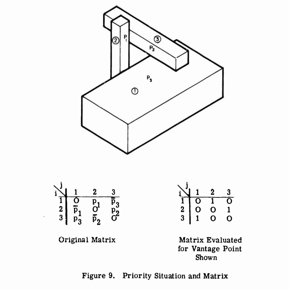
The researchers propose that this matrix could be implemented in hardware and re-evaluated every frame. Basically the matrix would act as a big switch or a kind of pre-built z-buffer. When drawing a given object, no video would be output for the parts of the object when a 1 exists in the object’s column and the corresponding row object is also being drawn.

The major drawback with this matrix approach is that to represent a scene with \(n\) objects you need a matrix of size \(n^2\). So the researchers go on to explore whether it would be feasible to represent the occlusion matrix as a “priority list” instead, which would only be of size \(n\) and would establish an order in which objects should be drawn. They immediately note that for certain scenes like the one in the figure above no ordering can be made (since there is an occlusion cycle), so they spend a lot of time laying out the mathematical distinction between “proper” and “improper” scenes. Eventually they conclude that, at least for “proper” scenes—and it should be easy enough for a scene designer to avoid “improper” cases—a priority list could be generated. But they leave the list generation as an exercise for the reader. It seems the primary contribution of this 1969 study was to point out that it should be possible to use partitioning planes to order objects in a scene for rendering, at least in theory.

It was not until 1980 that a paper, titled “On Visible Surface Generation by A Priori Tree Structures,” demonstrated a concrete algorithm to accomplish this. The 1980 paper, written by Henry Fuchs, Zvi Kedem, and Bruce Naylor, introduced the BSP tree. The authors say that their novel data structure is “an alternative solution to an approach first utilized a decade ago but due to a few difficulties, not widely exploited”—here referring to the approach taken in the 1969 Air Force study.3 A BSP tree, once constructed, can easily be used to provide a priority ordering for objects in the scene.

Fuchs, Kedem, and Naylor give a pretty readable explanation of how a BSP tree works, but let me see if I can provide a less formal but more concise one.

You begin by picking one polygon in your scene and making the plane in which the polygon lies your partitioning plane. That one polygon also ends up as the root node in your tree. The remaining polygons in your scene will be on one side or the other of your root partitioning plane. The polygons on the “forward” side or in the “forward” half-space of your plane end up in the left subtree of your root node, while the polygons on the “back” side or in the “back” half-space of your plane end up in the right subtree. You then repeat this process recursively, picking a polygon from your left and right subtrees to be the new partitioning planes for their respective half-spaces, which generates further half-spaces and further sub-trees. You stop when you run out of polygons.

Say you want to render the geometry in your scene from back-to-front. (This is known as the “painter’s algorithm,” since it means that polygons further from the camera will get drawn over by polygons closer to the camera, producing a correct rendering.) To achieve this, all you have to do is an in-order traversal of the BSP tree, where the decision to render the left or right subtree of any node first is determined by whether the camera viewpoint is in either the forward or back half-space relative to the partitioning plane associated with the node. So at each node in the tree, you render all the polygons on the “far” side of the plane first, then the polygon in the partitioning plane, then all the polygons on the “near” side of the plane—”far” and “near” being relative to the camera viewpoint. This solves the VSD problem because, as we learned several paragraphs back, the polygons on the far side of the partitioning plane cannot obstruct anything on the near side.

The following diagram shows the construction and traversal of a BSP tree representing a simple 2D scene. In 2D, the partitioning planes are instead partitioning lines, but the basic idea is the same in a more complicated 3D scene.

Step One: The root partitioning line along wall D splits the remaining geometry into two sets.

Step Two: The half-spaces on either side of D are split again. Wall C is the only wall in its half-space so no split is needed. Wall B forms the new partitioning line in its half-space. Wall A must be split into two walls since it crosses the partitioning line.

A back-to-front ordering of the walls relative to the viewpoint in the top-right corner, useful for implementing the painter’s algorithm. This is just an in-order traversal of the tree.

The really neat thing about a BSP tree, which Fuchs, Kedem, and Naylor stress several times, is that it only has to be constructed once. This is somewhat surprising, but the same BSP tree can be used to render a scene no matter where the camera viewpoint is. The BSP tree remains valid as long as the polygons in the scene don’t move. This is why the BSP tree is so useful for real-time rendering—all the hard work that goes into constructing the tree can be done beforehand rather than during rendering.

One issue that Fuchs, Kedem, and Naylor say needs further exploration is the question of what makes a “good” BSP tree. The quality of your BSP tree will depend on which polygons you decide to use to establish your partitioning planes. I skipped over this earlier, but if you partition using a plane that intersects other polygons, then in order for the BSP algorithm to work, you have to split the intersected polygons in two, so that one part can go in one half-space and the other part in the other half-space. If this happens a lot, then building a BSP tree will dramatically increase the number of polygons in your scene.

Bruce Naylor, one of the authors of the 1980 paper, would later write about this problem in his 1993 paper, “Constructing Good Partitioning Trees.” According to John Romero, one of Carmack’s fellow id Software co-founders, this paper was one of the papers that Carmack read when he was trying to implement BSP trees in Doom.4

BSP Trees in Doom

Remember that, in his first draft of the Doom renderer, Carmack had been trying to establish a rendering order for level geometry by “flooding” the renderer out from the player’s current room into neighboring rooms. BSP trees were a better way to establish this ordering because they avoided the issue where the renderer found itself visiting the same room (or sector) multiple times, wasting CPU cycles.

“Adding BSP trees to Doom” meant, in practice, adding a BSP tree generator to the Doom level editor. When a level in Doom was complete, a BSP tree was generated from the level geometry. According to Fabien Sanglard, the generation process could take as long as eight seconds for a single level and 11 minutes for all the levels in the original Doom.5 The generation process was lengthy in part because Carmack’s BSP generation algorithm tries to search for a “good” BSP tree using various heuristics. An eight-second delay would have been unforgivable at runtime, but it was not long to wait when done offline, especially considering the performance gains the BSP trees brought to the renderer. The generated BSP tree for a single level would have then ended up as part of the level data loaded into the game when it starts.

Carmack put a spin on the BSP tree algorithm outlined in the 1980 paper, because once Doom is started and the BSP tree for the current level is read into memory, the renderer uses the BSP tree to draw objects front-to-back rather than back-to-front. In the 1980 paper, Fuchs, Kedem, and Naylor show how a BSP tree can be used to implement the back-to-front painter’s algorithm, but the painter’s algorithm involves a lot of over-drawing that would have been expensive on an IBM-compatible PC. So the Doom renderer instead starts with the geometry closer to the player, draws that first, then draws the geometry farther away. This reverse ordering is easy to achieve using a BSP tree, since you can just make the opposite traversal decision at each node in the tree. To ensure that the farther-away geometry is not drawn over the closer geometry, the Doom renderer uses a kind of implicit z-buffer that provides much of the benefit of a z-buffer with a much smaller memory footprint. There is one array that keeps track of occlusion in the horizontal dimension, and another two arrays that keep track of occlusion in the vertical dimension from the top and bottom of the screen. The Doom renderer can get away with not using an actual z-buffer because Doom is not technically a fully 3D game. The cheaper data structures work because certain things never appear in Doom: The horizontal occlusion array works because there are no sloping walls, and the vertical occlusion arrays work because no walls have, say, two windows, one above the other.

The only other tricky issue left is how to incorporate Doom’s moving characters into the static level geometry drawn with the aid of the BSP tree. The enemies in Doom cannot be a part of the BSP tree because they move; the BSP tree only works for geometry that never moves. So the Doom renderer draws the static level geometry first, keeping track of the segments of the screen that were drawn to (with yet another memory-efficient data structure). It then draws the enemies in back-to-front order, clipping them against the segments of the screen that occlude them. This process is not as optimal as rendering using the BSP tree, but because there are usually fewer enemies visible than there is level geometry in a level, speed isn’t as much of an issue here.

Using BSP trees in Doom was a major win. Obviously it is pretty neat that Carmack was able to figure out that BSP trees were the perfect solution to his problem. But was it a genius-level move?

In his excellent book about the Doom game engine, Fabien Sanglard quotes John Romero saying that Bruce Naylor’s paper, “Constructing Good Partitioning Trees,” was mostly about using BSP trees to cull backfaces from 3D models.6 According to Romero, Carmack thought the algorithm could still be useful for Doom, so he went ahead and implemented it. This description is quite flattering to Carmack—it implies he saw that BSP trees could be useful for real-time video games when other people were still using the technique to render static scenes. There is a similarly flattering story in Masters of Doom: Kushner suggests that Carmack read Naylor’s paper and asked himself, “what if you could use a BSP to create not just one 3D image but an entire virtual world?”7

This framing ignores the history of the BSP tree. When those US Air Force researchers first realized that partitioning a scene might help speed up rendering, they were interested in speeding up real-time rendering, because they were, after all, trying to create a flight simulator. The flight simulator example comes up again in the 1980 BSP paper. Fuchs, Kedem, and Naylor talk about how a BSP tree would be useful in a flight simulator that pilots use to practice landing at the same airport over and over again. Since the airport geometry never changes, the BSP tree can be generated just once. Clearly what they have in mind is a real-time simulation. In the introduction to their paper, they even motivate their research by talking about how real-time graphics systems must be able to create an image in at least 1/30th of a second.

So Carmack was not the first person to think of using BSP trees in a real-time graphics simulation. Of course, it’s one thing to anticipate that BSP trees might be used this way and another thing to actually do it. But even in the implementation Carmack may have had more guidance than is commonly assumed. The [Wikipedia page about BSP
trees](https://en.wikipedia.org/wiki/Binary_space_partitioning), at least as of this writing, suggests that Carmack consulted a 1991 paper by Chen and Gordon as well as a 1990 textbook called Computer Graphics: Principles and Practice. Though no citation is provided for this claim, it is probably true. The 1991 Chen and Gordon paper outlines a front-to-back rendering approach using BSP trees that is basically the same approach taken by Doom, right down to what I’ve called the “implicit z-buffer” data structure that prevents farther polygons being drawn over nearer polygons. The textbook provides a great overview of BSP trees and some pseudocode both for building a tree and for displaying one. (I’ve been able to skim through the 1990 edition thanks to my wonderful university library.) Computer Graphics: Principles and Practice is a classic text in computer graphics, so Carmack might well have owned it.

Still, Carmack found himself faced with a novel problem—”How can we make a first-person shooter run on a computer with a CPU that can’t even do floating-point operations?”—did his research, and proved that BSP trees are a useful data structure for real-time video games. I still think that is an impressive feat, even if the BSP tree had first been invented a decade prior and was pretty well theorized by the time Carmack read about it. Perhaps the accomplishment that we should really celebrate is the Doom game engine as a whole, which is a seriously nifty piece of work. I’ve mentioned it once already, but Fabien Sanglard’s book about the Doom game engine ( Game Engine Black Book: DOOM) is an excellent overview of all the different clever components of the game engine and how they fit together. We shouldn’t forget that the VSD problem was just one of many problems that Carmack had to solve to make the Doom engine work. That he was able, on top of everything else, to read about and implement a complicated data structure unknown to most programmers speaks volumes about his technical expertise and his drive to perfect his craft.

If you enjoyed this post, more like it come out every four weeks! Follow @TwoBitHistory on Twitter or subscribe to the RSS feed to make sure you know when a new post is out.

Previously on TwoBitHistory…

I've wanted to learn more about GNU Readline for a while, so I thought I'd turn that into a new blog post. Includes a few fun facts from an email exchange with Chet Ramey, who maintains Readline (and Bash): https://t.co/wnXeuyjgMx

— TwoBitHistory (@TwoBitHistory) August 22, 2019

]]>Things You Didn’t Know About GNU Readline2019-08-22T00:00:00+00:002019-08-22T00:00:00+00:00https://twobithistory.org/2019/08/22/readlineI sometimes think of my computer as a very large house. I visit this house every day and know most of the rooms on the ground floor, but there are bedrooms I’ve never been in, closets I haven’t opened, nooks and crannies that I’ve never explored. I feel compelled to learn more about my computer the same way anyone would feel compelled to see a room they had never visited in their own home.

GNU Readline is an unassuming little software library that I relied on for years without realizing that it was there. Tens of thousands of people probably use it every day without thinking about it. If you use the Bash shell, every time you auto-complete a filename, or move the cursor around within a single line of input text, or search through the history of your previous commands, you are using GNU Readline. When you do those same things while using the command-line interface to Postgres ( psql), say, or the Ruby REPL ( irb), you are again using GNU Readline. Lots of software depends on the GNU Readline library to implement functionality that users expect, but the functionality is so auxiliary and unobtrusive that I imagine few people stop to wonder where it comes from.

GNU Readline was originally created in the 1980s by the Free Software Foundation. Today, it is an important if invisible part of everyone’s computing infrastructure, maintained by a single volunteer.

Feature Replete

The GNU Readline library exists primarily to augment any command-line interface with a common set of keystrokes that allow you to move around within and edit a single line of input. If you press Ctrl-A at a Bash prompt, for example, that will jump your cursor to the very beginning of the line, while pressing Ctrl-E will jump it to the end. Another useful command is Ctrl-U, which will delete everything in the line before the cursor.

For an embarrassingly long time, I moved around on the command line by repeatedly tapping arrow keys. For some reason, I never imagined that there was a faster way to do it. Of course, no programmer familiar with a text editor like Vim or Emacs would deign to punch arrow keys for long, so something like Readline was bound to be created. Using Readline, you can do much more than just jump around—you can edit your single line of text as if you were using a text editor. There are commands to delete words, transpose words, upcase words, copy and paste characters, etc. In fact, most of Readline’s keystrokes/shortcuts are based on Emacs. Readline is essentially Emacs for a single line of text. You can even record and replay macros.

I have never used Emacs, so I find it hard to remember what all the different Readline commands are. But one thing about Readline that is really neat is that you can switch to using a Vim-based mode instead. To do this for Bash, you can use the set builtin. The following will tell Readline to use Vim-style commands for the current shell:

With this option enabled, you can delete words using dw and so on. The equivalent to Ctrl-U in the Emacs mode would be d0.

I was excited to try this when I first learned about it, but I’ve found that it doesn’t work so well for me. I’m happy that this concession to Vim users exists, and you might have more luck with it than me, particularly if you haven’t already used Readline’s default command keystrokes. My problem is that, by the time I heard about the Vim-based interface, I had already learned several Readline keystrokes. Even with the Vim option enabled, I keep using the default keystrokes by mistake. Also, without some sort of indicator, Vim’s modal design is awkward here—it’s very easy to forget which mode you’re in. So I’m stuck at a local maximum using Vim as my text editor but Emacs-style Readline commands. I suspect a lot of other people are in the same position.

If you feel, not unreasonably, that both Vim and Emacs’ keyboard command systems are bizarre and arcane, you can customize Readline’s key bindings and make them whatever you like. This is not hard to do. Readline reads a ~/.inputrc file on startup that can be used to configure various options and key bindings. One thing I’ve done is reconfigured Ctrl-K. Normally it deletes from the cursor to the end of the line, but I rarely do that. So I’ve instead bound it so that pressing Ctrl-K deletes the whole line, regardless of where the cursor is. I’ve done that by adding the following to ~/.inputrc:

Control-k: kill-whole-line

Each Readline command (the documentation refers to them as functions) has a name that you can associate with a key sequence this way. If you edit ~/.inputrc in Vim, it turns out that Vim knows the filetype and will help you by highlighting valid function names but not invalid ones!

Another thing you can do with ~/.inputrc is create canned macros by mapping key sequences to input strings. [The Readline
manual](https://tiswww.case.edu/php/chet/readline/readline.html) gives one example that I think is especially useful. I often find myself wanting to save the output of a program to a file, which means that I often append something like > output.txt to Bash commands. To save some time, you could make this a Readline macro:

Control-o: "> output.txt"

Now, whenever you press Ctrl-O, you’ll see that > output.txt gets added after your cursor on the command line. Neat!

But with macros you can do more than just create shortcuts for strings of text. The following entry in ~/.inputrc means that, every time I press Ctrl-J, any text I already have on the line is surrounded by $( and ). The macro moves to the beginning of the line with Ctrl-A, adds $(, then moves to the end of the line with Ctrl-E and adds ):

This might be useful if you often need the output of one command to use for another, such as in:

The ~/.inputrc file also allows you to set different values for what the Readline manual calls variables. These enable or disable certain Readline behaviors. You can use these variables to change, for example, how Readline auto-completion works or how the Readline history search works. One variable I’d recommend turning on is the revert-all-at-newline variable, which by default is off. When the variable is off, if you pull a line from your command history using the reverse search feature, edit it, but then decide to search instead for another line, the edit you made is preserved in the history. I find this confusing because it leads to lines showing up in your Bash command history that you never actually ran. So add this to your ~/.inputrc:

set revert-all-at-newline on

When you set options or key bindings using ~/.inputrc, they apply wherever the Readline library is used. This includes Bash most obviously, but you’ll also get the benefit of your changes in other programs like irb and psql too! A Readline macro that inserts SELECT * FROM could be useful if you often use command-line interfaces to relational databases.

Chet Ramey

GNU Readline is today maintained by Chet Ramey, a Senior Technology Architect at Case Western Reserve University. Ramey also maintains the Bash shell. Both projects were first authored by a Free Software Foundation employee named Brian Fox beginning in 1988. But Ramey has been the sole maintainer since around 1994.

Ramey told me via email that Readline, far from being an original idea, was created to implement functionality prescribed by the POSIX specification, which in the late 1980s had just been created. Many earlier shells, including the Korn shell and at least one version of the Unix System V shell, included line editing functionality. The 1988 version of the Korn shell ( ksh88) provided both Emacs-style and Vi/Vim-style editing modes. As far as I can tell from [the
manual
page](https://web.archive.org/web/20151105130220/http://www2.research.att.com/sw/download/man/man1/ksh88.html), the Korn shell would decide which mode you wanted to use by looking at the VISUAL and EDITOR environment variables, which is pretty neat. The parts of POSIX that specified shell functionality were closely modeled on ksh88, so GNU Bash was going to have to implement a similarly flexible line-editing system to stay compliant. Hence Readline.

When Ramey first got involved in Bash development, Readline was a single source file in the Bash project directory. It was really just a part of Bash. Over time, the Readline file slowly moved toward becoming an independent project, though it was not until 1994 (with the 2.0 release of Readline) that Readline became a separate library entirely.

Readline is closely associated with Bash, and Ramey usually pairs Readline releases with Bash releases. But as I mentioned above, Readline is a library that can be used by any software implementing a command-line interface. And it’s really easy to use. This is a simple example, but here’s how you would you use Readline in your own C program. The string argument to the readline() function is the prompt that you want Readline to display to the user:

#include <stdio.h>
#include <stdlib.h>
#include "readline/readline.h"

int main(int argc, char** argv)
{
    char* line = readline("my-rl-example> ");
    printf("You entered: \"%s\"\n", line);

    free(line);

    return 0;
}

Your program hands off control to Readline, which is responsible for getting a line of input from the user (in such a way that allows the user to do all the fancy line-editing things). Once the user has actually submitted the line, Readline returns it to you. I was able to compile the above by linking against the Readline library, which I apparently have somewhere in my library search path, by invoking the following:

The Readline API is much more extensive than that single function of course, and anyone using it can tweak all sorts of things about the library’s behavior. Library users can even add new functions that end users can configure via ~/.inputrc, meaning that Readline is very easy to extend. But, as far as I can tell, even Bash ultimately calls the simple readline() function to get input just as in the example above, though there is a lot of configuration beforehand. (See [this
line](https://github.com/bminor/bash/blob/9f597fd10993313262cab400bf3c46ffb3f6fd1e/parse.y#L1487) in the source for GNU Bash, which seems to be where Bash hands off responsibility for getting input to Readline.)

Ramey has now worked on Bash and Readline for well over a decade. He has never once been compensated for his work—he is and has always been a volunteer. Bash and Readline continue to be actively developed, though Ramey said that Readline changes much more slowly than Bash does. I asked Ramey what it was like being the sole maintainer of software that so many people use. He said that millions of people probably use Bash without realizing it (because every Apple device runs Bash), which makes him worry about how much disruption a breaking change might cause. But he’s slowly gotten used to the idea of all those people out there. He said that he continues to work on Bash and Readline because at this point he is deeply invested and because he simply likes to make useful software available to the world.

You can find more information about Chet Ramey at his_ _website.

If you enjoyed this post, more like it come out every four weeks! Follow @TwoBitHistory on Twitter or subscribe to the RSS feed to make sure you know when a new post is out.

Previously on TwoBitHistory…

Please enjoy my long overdue new post, in which I use the story of the BBC Micro and the Computer Literacy Project as a springboard to complain about Codecademy. https://t.co/PiWlKljDjK

— TwoBitHistory (@TwoBitHistory) March 31, 2019

]]>Codecademy vs. The BBC Micro2019-03-31T00:00:00+00:002019-03-31T00:00:00+00:00https://twobithistory.org/2019/03/31/bbc-microIn the late 1970s, the computer, which for decades had been a mysterious, hulking machine that only did the bidding of corporate overlords, suddenly became something the average person could buy and take home. An enthusiastic minority saw how great this was and rushed to get a computer of their own. For many more people, the arrival of the microcomputer triggered helpless anxiety about the future. An ad from a magazine at the time promised that a home computer would “give your child an unfair advantage in school.” It showed a boy in a smart blazer and tie eagerly raising his hand to answer a question, while behind him his dim-witted classmates look on sullenly. The ad and others like it implied that the world was changing quickly and, if you did not immediately learn how to use one of these intimidating new devices, you and your family would be left behind.

In the UK, this anxiety metastasized into concern at the highest levels of government about the competitiveness of the nation. The 1970s had been, on the whole, an underwhelming decade for Great Britain. Both inflation and unemployment had been high. Meanwhile, a series of strikes put London through blackout after blackout. A government report from 1979 fretted that a failure to keep up with trends in computing technology would “add another factor to our poor industrial performance.”1 The country already seemed to be behind in the computing arena—all the great computer companies were American, while integrated circuits were being assembled in Japan and Taiwan.

In an audacious move, the BBC, a public service broadcaster funded by the government, decided that it would solve Britain’s national competitiveness problems by helping Britons everywhere overcome their aversion to computers. It launched the Computer Literacy Project, a multi-pronged educational effort that involved several TV series, a few books, a network of support groups, and a specially built microcomputer known as the BBC Micro. The project was so successful that, by 1983, an editor for BYTE Magazine wrote, “compared to the US, proportionally more of Britain’s population is interested in microcomputers.”2 The editor marveled that there were more people at the Fifth Personal Computer World Show in the UK than had been to that year’s West Coast Computer Faire. Over a sixth of Great Britain watched an episode in the first series produced for the Computer Literacy Project and 1.5 million BBC Micros were ultimately sold.3

[An
archive](https://computer-literacy-project.pilots.bbcconnectedstudio.co.uk/) containing every TV series produced and all the materials published for the Computer Literacy Project was put on the web last year. I’ve had a huge amount of fun watching the TV series and trying to imagine what it would have been like to learn about computing in the early 1980s. But what’s turned out to be more interesting is how computing was taught. Today, we still worry about technology leaving people behind. Wealthy tech entrepreneurs and governments spend lots of money trying to teach kids “to code.” We have websites like Codecademy that make use of new technologies to teach coding interactively. One would assume that this approach is more effective than a goofy ’80s TV series. But is it?

The Computer Literacy Project

The microcomputer revolution began in 1975 with the release of [the Altair
8800](https://twobithistory.org/2018/07/22/dawn-of-the-microcomputer.html). Only two years later, the Apple II, TRS-80, and Commodore PET had all been released. Sales of the new computers exploded. In 1978, the BBC explored the dramatic societal changes these new machines were sure to bring in a documentary called “Now the Chips Are Down.”

The documentary was alarming. Within the first five minutes, the narrator explains that microelectronics will “totally revolutionize our way of life.” As eerie synthesizer music plays, and green pulses of electricity dance around a magnified microprocessor on screen, the narrator argues that the new chips are why “Japan is abandoning its ship building, and why our children will grow up without jobs to go to.” The documentary goes on to explore how robots are being used to automate car assembly and how the European watch industry has lost out to digital watch manufacturers in the United States. It castigates the British government for not doing more to prepare the country for a future of mass unemployment.

The documentary was supposedly shown to the British Cabinet.4 Several government agencies, including the Department of Industry and the Manpower Services Commission, became interested in trying to raise awareness about computers among the British public. The Manpower Services Commission provided funds for a team from the BBC’s education division to travel to Japan, the United States, and other countries on a fact-finding trip. This research team produced a report that cataloged the ways in which microelectronics would indeed mean major changes for industrial manufacturing, labor relations, and office work. In late 1979, it was decided that the BBC should make a ten-part TV series that would help regular Britons “learn how to use and control computers and not feel dominated by them.”5 The project eventually became a multimedia endeavor similar to the Adult Literacy Project, an earlier BBC undertaking involving both a TV series and supplemental courses that helped two million people improve their reading.

The producers behind the Computer Literacy Project were keen for the TV series to feature “hands-on” examples that viewers could try on their own if they had a microcomputer at home. These examples would have to be in BASIC, since that was the language (really the entire shell) used on almost all microcomputers. But the producers faced a thorny problem: Microcomputer manufacturers all had their own dialects of BASIC, so no matter which dialect they picked, they would inevitably alienate some large fraction of their audience. The only real solution was to create a new BASIC—BBC BASIC—and a microcomputer to go along with it. Members of the British public would be able to buy the new microcomputer and follow along without worrying about differences in software or hardware.

The TV producers and presenters at the BBC were not capable of building a microcomputer on their own. So they put together a specification for the computer they had in mind and invited British microcomputer companies to propose a new machine that met the requirements. The specification called for a relatively powerful computer because the BBC producers felt that the machine should be able to run real, useful applications. Technical consultants for the Computer Literacy Project also suggested that, if it had to be a BASIC dialect that was going to be taught to the entire nation, then it had better be a good one. (They may not have phrased it exactly that way, but I bet that’s what they were thinking.) BBC BASIC would make up for some of BASIC’s usual shortcomings by allowing for recursion and local variables.6

The BBC eventually decided that a Cambridge-based company called Acorn Computers would make the BBC Micro. In choosing Acorn, the BBC passed over a proposal from Clive Sinclair, who ran a company called Sinclair Research. Sinclair Research had brought mass-market microcomputing to the UK in 1980 with the Sinclair ZX80. Sinclair’s new computer, the ZX81, was cheap but not powerful enough for the BBC’s purposes. Acorn’s new prototype computer, known internally as the Proton, would be more expensive but more powerful and expandable. The BBC was impressed. The Proton was never marketed or sold as the Proton because it was instead released in December 1981 as the BBC Micro, also affectionately called “The Beeb.” You could get a 16k version for £235 and a 32k version for £335.

In 1980, Acorn was an underdog in the British computing industry. But the BBC Micro helped establish the company’s legacy. Today, the world’s most popular microprocessor instruction set is the ARM architecture. “ARM” now stands for “Advanced RISC Machine,” but originally it stood for “Acorn RISC Machine.” ARM Holdings, the company behind the architecture, was spun out from Acorn in 1990.

A bad picture of a BBC Micro, taken by me at the Computer History Museum

in Mountain View, California.

The Computer Programme

A dozen different TV series were eventually produced as part of the Computer Literacy Project, but the first of them was a ten-part series known as The Computer Programme. The series was broadcast over ten weeks at the beginning of 1982. A million people watched each week-night broadcast of the show; a quarter million watched the reruns on Sunday and Monday afternoon.

The show was hosted by two presenters, Chris Serle and Ian McNaught-Davis. Serle plays the neophyte while McNaught-Davis, who had professional experience programming mainframe computers, plays the expert. This was an inspired setup. It made for [awkward
transitions](https://twitter.com/TwoBitHistory/status/1112372000742404098)—Serle often goes directly from a conversation with McNaught-Davis to a bit of walk-and-talk narration delivered to the camera, and you can’t help but wonder whether McNaught-Davis is still standing there out of frame or what. But it meant that Serle could voice the concerns that the audience would surely have. He can look intimidated by a screenful of BASIC and can ask questions like, “What do all these dollar signs mean?” At several points during the show, Serle and McNaught-Davis sit down in front of a computer and essentially pair program, with McNaught-Davis providing hints here and there while Serle tries to figure it out. It would have been much less relatable if the show had been presented by a single, all-knowing narrator.

The show also made an effort to demonstrate the many practical applications of computing in the lives of regular people. By the early 1980s, the home computer had already begun to be associated with young boys and video games. The producers behind The Computer Programme sought to avoid interviewing “impressively competent youngsters,” as that was likely “to increase the anxieties of older viewers,” a demographic that the show was trying to attract to computing.7 In the first episode of the series, Gill Nevill, the show’s “on location” reporter, interviews a woman that has bought a Commodore PET to help manage her sweet shop. The woman (her name is Phyllis) looks to be 60-something years old, yet she has no trouble using the computer to do her accounting and has even started using her PET to do computer work for other businesses, which sounds like the beginning of a promising freelance career. Phyllis says that she wouldn’t mind if the computer work grew to replace her sweet shop business since she enjoys the computer work more. This interview could instead have been an interview with a teenager about how he had modified Breakout to be faster and more challenging. But that would have been encouraging to almost nobody. On the other hand, if Phyllis, of all people, can use a computer, then surely you can too.

While the show features lots of BASIC programming, what it really wants to teach its audience is how computing works in general. The show explains these general principles with analogies. In the second episode, there is an extended discussion of the Jacquard loom, which accomplishes two things. First, it illustrates that computers are not based only on magical technology invented yesterday—some of the foundational principles of computing go back two hundred years and are about as simple as the idea that you can punch holes in card to control a weaving machine. Second, the interlacing of warp and weft threads is used to demonstrate how a binary choice (does the weft thread go above or below the warp thread?) is enough, when repeated over and over, to produce enormous variation. This segues, of course, into a discussion of how information can be stored using binary digits.

Later in the show there is a section about a steam organ that plays music encoded in a long, segmented roll of punched card. This time the analogy is used to explain subroutines in BASIC. Serle and McNaught-Davis lay out the whole roll of punched card on the floor in the studio, then point out the segments where it looks like a refrain is being repeated. McNaught-Davis explains that a subroutine is what you would get if you cut out those repeated segments of card and somehow added an instruction to go back to the original segment that played the refrain for the first time. This is a brilliant explanation and probably one that stuck around in people’s minds for a long time afterward.

I’ve picked out only a few examples, but I think in general the show excels at demystifying computers by explaining the principles that computers rely on to function. The show could instead have focused on teaching BASIC, but it did not. This, it turns out, was very much a conscious choice. In a retrospective written in 1983, John Radcliffe, the executive producer of the Computer Literacy Project, wrote the following:

If computers were going to be as important as we believed, some genuine understanding of this new subject would be important for everyone, almost as important perhaps as the capacity to read and write. Early ideas, both here and in America, had concentrated on programming as the main route to computer literacy. However, as our thinking progressed, although we recognized the value of “hands-on” experience on personal micros, we began to place less emphasis on programming and more on wider understanding, on relating micros to larger machines, encouraging people to gain experience with a range of applications programs and high-level languages, and relating these to experience in the real world of industry and commerce…. Our belief was that once people had grasped these principles, at their simplest, they would be able to move further forward into the subject.

Later, Radcliffe writes, in a similar vein:

There had been much debate about the main explanatory thrust of the series. One school of thought had argued that it was particularly important for the programmes to give advice on the practical details of learning to use a micro. But we had concluded that if the series was to have any sustained educational value, it had to be a way into the real world of computing, through an explanation of computing principles. This would need to be achieved by a combination of studio demonstration on micros, explanation of principles by analogy, and illustration on film of real-life examples of practical applications. Not only micros, but mini computers and mainframes would be shown.

I love this, particularly the part about mini-computers and mainframes. The producers behind The Computer Programme aimed to help Britons get situated: Where had computing been, and where was it going? What can computers do now, and what might they do in the future? Learning some BASIC was part of answering those questions, but knowing BASIC alone was not seen as enough to make someone computer literate.

Computer Literacy Today

If you google “learn to code,” the first result you see is a link to Codecademy’s website. If there is a modern equivalent to the Computer Literacy Project, something with the same reach and similar aims, then it is Codecademy.

“Learn to code” is Codecademy’s tagline. I don’t think I’m the first person to point this out—in fact, I probably read this somewhere and I’m now ripping it off—but there’s something revealing about using the word “code” instead of “program.” It suggests that the important thing you are learning is how to decode the code, how to look at a screen’s worth of Python and not have your eyes glaze over. I can understand why to the average person this seems like the main hurdle to becoming a professional programmer. Professional programmers spend all day looking at computer monitors covered in gobbledygook, so, if I want to become a professional programmer, I better make sure I can decipher the gobbledygook. But dealing with syntax is not the most challenging part of being a programmer, and it quickly becomes almost irrelevant in the face of much bigger obstacles. Also, armed only with knowledge of a programming language’s syntax, you may be able to read code but you won’t be able to write code to solve a novel problem.

I recently went through Codecademy’s “Code Foundations” course, which is the course that the site recommends you take if you are interested in programming (as opposed to web development or data science) and have never done any programming before. There are a few lessons in there about the history of computer science, but they are perfunctory and poorly researched. (Thank heavens for [this noble internet
vigilante](https://twitter.com/TwoBitHistory/status/1111305774939234304), who pointed out a particularly egregious error.) The main focus of the course is teaching you about the common structural elements of programming languages: variables, functions, control flow, loops. In other words, the course focuses on what you would need to know to start seeing patterns in the gobbledygook.

To be fair to Codecademy, they offer other courses that look meatier. But even courses such as their “Computer Science Path” course focus almost exclusively on programming and concepts that can be represented in programs. One might argue that this is the whole point—Codecademy’s main feature is that it gives you little interactive programming lessons with automated feedback. There also just isn’t enough room to cover more because there is only so much you can stuff into somebody’s brain in a little automated lesson. But the producers at the BBC tasked with kicking off the Computer Literacy Project also had this problem; they recognized that they were limited by their medium and that “the amount of learning that would take place as a result of the television programmes themselves would be limited.”8 With similar constraints on the volume of information they could convey, they chose to emphasize general principles over learning BASIC. Couldn’t Codecademy replace a lesson or two with an interactive visualization of a Jacquard loom weaving together warp and weft threads?

I’m banging the drum for “general principles” loudly now, so let me just explain what I think they are and why they are important. There’s a book by J. Clark Scott about computers called But How Do It Know? The title comes from the anecdote that opens the book. A salesman is explaining to a group of people that a thermos can keep hot food hot and cold food cold. A member of the audience, astounded by this new invention, asks, “But how do it know?” The joke of course is that the thermos is not perceiving the temperature of the food and then making a decision—the thermos is just constructed so that cold food inevitably stays cold and hot food inevitably stays hot. People anthropomorphize computers in the same way, believing that computers are digital brains that somehow “choose” to do one thing or another based on the code they are fed. But learning a few things about how computers work, even at a rudimentary level, takes the homunculus out of the machine. That’s why the Jacquard loom is such a good go-to illustration. It may at first seem like an incredible device. It reads punch cards and somehow “knows” to weave the right pattern! The reality is mundane: Each row of holes corresponds to a thread, and where there is a hole in that row the corresponding thread gets lifted. Understanding this may not help you do anything new with computers, but it will give you the confidence that you are not dealing with something magical. We should impart this sense of confidence to beginners as soon as we can.

Alas, it’s possible that the real problem is that nobody wants to learn about the Jacquard loom. Judging by how Codecademy emphasizes the professional applications of what it teaches, many people probably start using Codecademy because they believe it will help them “level up” their careers. They believe, not unreasonably, that the primary challenge will be understanding the gobbledygook, so they want to “learn to code.” And they want to do it as quickly as possible, in the hour or two they have each night between dinner and collapsing into bed. Codecademy, which after all is a business, gives these people what they are looking for—not some roundabout explanation involving a machine invented in the 18th century.

The Computer Literacy Project, on the other hand, is what a bunch of producers and civil servants at the BBC thought would be the best way to educate the nation about computing. I admit that it is a bit elitist to suggest we should laud this group of people for teaching the masses what they were incapable of seeking out on their own. But I can’t help but think they got it right. Lots of people first learned about computing using a BBC Micro, and many of these people went on to become successful software developers or game designers. As I’ve written before, I suspect learning about computing at a time when computers were relatively simple was a huge advantage. But perhaps another advantage these people had is shows like The Computer Programme, which strove to teach not just programming but also how and why computers can run programs at all. After watching The Computer Programme, you may not understand all the gobbledygook on a computer screen, but you don’t really need to because you know that, whatever the “code” looks like, the computer is always doing the same basic thing. After a course or two on Codecademy, you understand some flavors of gobbledygook, but to you a computer is just a magical machine that somehow turns gobbledygook into running software. That isn’t computer literacy.

If you enjoyed this post, more like it come out every four weeks! Follow @TwoBitHistory on Twitter or subscribe to the RSS feed to make sure you know when a new post is out.

Previously on TwoBitHistory…

FINALLY some new damn content, amirite?

Wanted to write an article about how Simula bought us object-oriented programming. It did that, but early Simula also flirted with a different vision for how OOP would work. Wrote about that instead! https://t.co/AYIWRRceI6

— TwoBitHistory (@TwoBitHistory) February 1, 2019

]]>OOP Before OOP with Simula2019-01-31T00:00:00+00:002019-01-31T00:00:00+00:00https://twobithistory.org/2019/01/31/simulaImagine that you are sitting on the grassy bank of a river. Ahead of you, the water flows past swiftly. The afternoon sun has put you in an idle, philosophical mood, and you begin to wonder whether the river in front of you really exists at all. Sure, large volumes of water are going by only a few feet away. But what is this thing that you are calling a “river”? After all, the water you see is here and then gone, to be replaced only by more and different water. It doesn’t seem like the word “river” refers to any fixed thing in front of you at all.

In 2009, Rich Hickey, the creator of Clojure, gave [an excellent
talk](https://www.infoq.com/presentations/Are-We-There-Yet-Rich-Hickey) about why this philosophical quandary poses a problem for the object-oriented programming paradigm. He argues that we think of an object in a computer program the same way we think of a river—we imagine that the object has a fixed identity, even though many or all of the object’s properties will change over time. Doing this is a mistake, because we have no way of distinguishing between an object instance in one state and the same object instance in another state. We have no explicit notion of time in our programs. We just breezily use the same name everywhere and hope that the object is in the state we expect it to be in when we reference it. Inevitably, we write bugs.

The solution, Hickey concludes, is that we ought to model the world not as a collection of mutable objects but a collection of processes acting on immutable data. We should think of each object as a “river” of causally related states. In sum, you should use a functional language like Clojure.

The author, on a hike, pondering the ontological commitments

of object-oriented programming.

Since Hickey gave his talk in 2009, interest in functional programming languages has grown, and functional programming idioms have found their way into the most popular object-oriented languages. Even so, most programmers continue to instantiate objects and mutate them in place every day. And they have been doing it for so long that it is hard to imagine that programming could ever look different.

I wanted to write an article about Simula and imagined that it would mostly be about when and how object-oriented constructs we are familiar with today were added to the language. But I think the more interesting story is about how Simula was originally so unlike modern object-oriented programming languages. This shouldn’t be a surprise, because the object-oriented paradigm we know now did not spring into existence fully formed. There were two major versions of Simula: Simula I and Simula 67. Simula 67 brought the world classes, class hierarchies, and virtual methods. But Simula I was a first draft that experimented with other ideas about how data and procedures could be bundled together. The Simula I model is not a functional model like the one Hickey proposes, but it does focus on processes that unfold over time rather than objects with hidden state that interact with each other. Had Simula 67 stuck with more of Simula I’s ideas, the object-oriented paradigm we know today might have looked very different indeed—and that contingency should teach us to be wary of assuming that the current paradigm will dominate forever.

Simula 0 Through 67

Simula was created by two Norwegians, Kristen Nygaard and Ole-Johan Dahl.

In the late 1950s, Nygaard was employed by the Norwegian Defense Research Establishment (NDRE), a research institute affiliated with the Norwegian military. While there, he developed Monte Carlo simulations used for nuclear reactor design and operations research. These simulations were at first done by hand and then eventually programmed and run on a Ferranti Mercury.1 Nygaard soon found that he wanted a higher-level way to describe these simulations to a computer.

The kind of simulation that Nygaard commonly developed is known as a “discrete event model.” The simulation captures how a sequence of events change the state of a system over time—but the important property here is that the simulation can jump from one event to the next, since the events are discrete and nothing changes in the system between events. This kind of modeling, according to a paper that Nygaard and Dahl presented about Simula in 1966, was increasingly being used to analyze “nerve networks, communication systems, traffic flow, production systems, administrative systems, social systems, etc.”2 So Nygaard thought that other people might want a higher-level way to describe these simulations too. He began looking for someone that could help him implement what he called his “Simulation Language” or “Monte Carlo Compiler.”3

Dahl, who had also been employed by NDRE, where he had worked on language design, came aboard at this point to play Wozniak to Nygaard’s Jobs. Over the next year or so, Nygaard and Dahl worked to develop what has been called “Simula 0.”4 This early version of the language was going to be merely a modest extension to ALGOL 60, and the plan was to implement it as a preprocessor. The language was then much less abstract than what came later. The primary language constructs were “stations” and “customers.” These could be used to model certain discrete event networks; Nygaard and Dahl give an example simulating airport departures.5 But Nygaard and Dahl eventually came up with a more general language construct that could represent both “stations” and “customers” and also model a wider range of simulations. This was the first of two major generalizations that took Simula from being an application-specific ALGOL package to a general-purpose programming language.

In Simula I, there were no “stations” or “customers,” but these could be recreated using “processes.” A process was a bundle of data attributes associated with a single action known as the process’ operating rule. You might think of a process as an object with only a single method, called something like run(). This analogy is imperfect though, because each process’ operating rule could be suspended or resumed at any time—the operating rules were a kind of coroutine. A Simula I program would model a system as a set of processes that conceptually all ran in parallel. Only one process could actually be “current” at any time, but once a process suspended itself the next queued process would automatically take over. As the simulation ran, behind the scenes, Simula would keep a timeline of “event notices” that tracked when each process should be resumed. In order to resume a suspended process, Simula needed to keep track of multiple call stacks. This meant that Simula could no longer be an ALGOL preprocessor, because ALGOL had only once call stack. Nygaard and Dahl were committed to writing their own compiler.

In their paper introducing this system, Nygaard and Dahl illustrate its use by implementing a simulation of a factory with a limited number of machines that can serve orders.6 The process here is the order, which starts by looking for an available machine, suspends itself to wait for one if none are available, and then runs to completion once a free machine is found. There is a definition of the order process that is then used to instantiate several different order instances, but no methods are ever called on these instances. The main part of the program just creates the processes and sets them running.

The first Simula I compiler was finished in 1965. The language grew popular at the Norwegian Computer Center, where Nygaard and Dahl had gone to work after leaving NDRE. Implementations of Simula I were made available to UNIVAC users and to Burroughs B5500 users.7 Nygaard and Dahl did a consulting deal with a Swedish company called ASEA that involved using Simula to run job shop simulations. But Nygaard and Dahl soon realized that Simula could be used to write programs that had nothing to do with simulation at all.

Stein Krogdahl, a professor at the University of Oslo that has written about the history of Simula, claims that “the spark that really made the development of a new general-purpose language take off” was [a paper called “Record
Handling”](https://archive.computerhistory.org/resources/text/algol/ACM_Algol_bulletin/1061032/p39-hoare.pdf) by the British computer scientist C.A.R. Hoare.8 If you read Hoare’s paper now, this is easy to believe. I’m surprised that you don’t hear Hoare’s name more often when people talk about the history of object-oriented languages. Consider this excerpt from his paper:

The proposal envisages the existence inside the computer during the execution of the program, of an arbitrary number of records, each of which represents some object which is of past, present or future interest to the programmer. The program keeps dynamic control of the number of records in existence, and can create new records or destroy existing ones in accordance with the requirements of the task in hand.

Each record in the computer must belong to one of a limited number of disjoint record classes; the programmer may declare as many record classes as he requires, and he associates with each class an identifier to name it. A record class name may be thought of as a common generic term like “cow,” “table,” or “house” and the records which belong to these classes represent the individual cows, tables, and houses.

Hoare does not mention subclasses in this particular paper, but Dahl credits him with introducing Nygaard and himself to the concept.9 Nygaard and Dahl had noticed that processes in Simula I often had common elements. Using a superclass to implement those common elements would be convenient. This also raised the possibility that the “process” idea itself could be implemented as a superclass, meaning that not every class had to be a process with a single operating rule. This then was the second great generalization that would make Simula 67 a truly general-purpose programming language. It was such a shift of focus that Nygaard and Dahl briefly considered changing the name of the language so that people would know it was not just for simulations.10 But “Simula” was too much of an established name for them to risk it.

In 1967, Nygaard and Dahl signed a contract with Control Data to implement this new version of Simula, to be known as Simula 67. A conference was held in June, where people from Control Data, the University of Oslo, and the Norwegian Computing Center met with Nygaard and Dahl to establish a specification for this new language. This conference eventually led to a document called the [“Simula 67 Common Base
Language,”](http://web.eah-jena.de/~kleine/history/languages/Simula-CommonBaseLanguage.pdf) which defined the language going forward.

Several different vendors would make Simula 67 compilers. The Association of Simula Users (ASU) was founded and began holding annual conferences. Simula 67 soon had users in more than 23 different countries.11

21st Century Simula

Simula is remembered now because of its influence on the languages that have supplanted it. You would be hard-pressed to find anyone still using Simula to write application programs. But that doesn’t mean that Simula is an entirely dead language. You can still compile and run Simula programs on your computer today, thanks to GNU cim.

The cim compiler implements the Simula standard as it was after a revision in 1986. But this is mostly the Simula 67 version of the language. You can write classes, subclass, and virtual methods just as you would have with Simula 67. So you could create a small object-oriented program that looks a lot like something you could easily write in Python or Ruby:

! dogs.sim ;
Begin
    Class Dog;
        ! The cim compiler requires virtual procedures to be fully specified ;
        Virtual: Procedure bark Is Procedure bark;;
    Begin
        Procedure bark;
        Begin
            OutText("Woof!");
            OutImage;           ! Outputs a newline ;
        End;
    End;

    Dog Class Chihuahua;        ! Chihuahua is "prefixed" by Dog ;
    Begin
        Procedure bark;
        Begin
            OutText("Yap yap yap yap yap yap");
            OutImage;
        End;
    End;

    Ref (Dog) d;
    d :- new Chihuahua;         ! :- is the reference assignment operator ;
    d.bark;
End;

You would compile and run it as follows:

$ cim dogs.sim
Compiling dogs.sim:
gcc -g -O2 -c dogs.c
gcc -g -O2 -o dogs dogs.o -L/usr/local/lib -lcim
$ ./dogs
Yap yap yap yap yap yap

(You might notice that cim compiles Simula to C, then hands off to a C compiler.)

This was what object-oriented programming looked like in 1967, and I hope you agree that aside from syntactic differences this is also what object-oriented programming looks like in 2019. So you can see why Simula is considered a historically important language.

But I’m more interested in showing you the process model that was central to Simula I. That process model is still available in Simula 67, but only when you use the Process class and a special Simulation block.

In order to show you how processes work, I’ve decided to simulate the following scenario. Imagine that there is a village full of villagers next to a river. The river has lots of fish, but between them the villagers only have one fishing rod. The villagers, who have voracious appetites, get hungry every 60 minutes or so. When they get hungry, they have to use the fishing rod to catch a fish. If a villager cannot use the fishing rod because another villager is waiting for it, then the villager queues up to use the fishing rod. If a villager has to wait more than five minutes to catch a fish, then the villager loses health. If a villager loses too much health, then that villager has starved to death.

This is a somewhat strange example and I’m not sure why this is what first came to mind. But there you go. We will represent our villagers as Simula processes and see what happens over a day’s worth of simulated time in a village with four villagers.

The full program is [available here as a
Gist](https://gist.github.com/sinclairtarget/6364cd521010d28ee24dd41ab3d61a96).

The last lines of my output look like the following. Here we are seeing what happens in the last few hours of the day:

1299.45: John is hungry and requests the fishing rod.
1299.45: John is now fishing.
1311.39: John has caught a fish.
1328.96: Betty is hungry and requests the fishing rod.
1328.96: Betty is now fishing.
1331.25: Jane is hungry and requests the fishing rod.
1340.44: Betty has caught a fish.
1340.44: Jane went hungry waiting for the rod.
1340.44: Jane starved to death waiting for the rod.
1369.21: John is hungry and requests the fishing rod.
1369.21: John is now fishing.
1379.33: John has caught a fish.
1409.59: Betty is hungry and requests the fishing rod.
1409.59: Betty is now fishing.
1419.98: Betty has caught a fish.
1427.53: John is hungry and requests the fishing rod.
1427.53: John is now fishing.
1437.52: John has caught a fish.

Poor Jane starved to death. But she lasted longer than Sam, who didn’t even make it to 7am. Betty and John sure have it good now that only two of them need the fishing rod.

What I want you to see here is that the main, top-level part of the program does nothing but create the four villager processes and get them going. The processes manipulate the fishing rod object in the same way that we would manipulate an object today. But the main part of the program does not call any methods or modify and properties on the processes. The processes have internal state, but this internal state only gets modified by the process itself.

There are still fields that get mutated in place here, so this style of programming does not directly address the problems that pure functional programming would solve. But as Krogdahl observes, “this mechanism invites the programmer of a simulation to model the underlying system as a set of processes, each describing some natural sequence of events in that system.”12 Rather than thinking primarily in terms of nouns or actors—objects that do things to other objects—here we are thinking of ongoing processes. The benefit is that we can hand overall control of our program off to Simula’s event notice system, which Krogdahl calls a “time manager.” So even though we are still mutating processes in place, no process makes any assumptions about the state of another process. Each process interacts with other processes only indirectly.

It’s not obvious how this pattern could be used to build, say, a compiler or an HTTP server. (On the other hand, if you’ve ever programmed games in the Unity game engine, this should look familiar.) I also admit that even though we have a “time manager” now, this may not have been exactly what Hickey meant when he said that we need an explicit notion of time in our programs. (I think he’d want something like the superscript notation that Ada Lovelace used to distinguish between the different values a variable assumes through time.) All the same, I think it’s really interesting that right there at the beginning of object-oriented programming we can find a style of programming that is not all like the object-oriented programming we are used to. We might take it for granted that object-oriented programming simply works one way—that a program is just a long list of the things that certain objects do to other objects in the exact order that they do them. Simula I’s process system shows that there are other approaches. Functional languages are probably a better thought-out alternative, but Simula I reminds us that the very notion of alternatives to modern object-oriented programming should come as no surprise.

If you enjoyed this post, more like it come out every four weeks! Follow @TwoBitHistory on Twitter or subscribe to the RSS feed to make sure you know when a new post is out.

Previously on TwoBitHistory…

Hey everyone! I sadly haven't had time to do any new writing but I've just put up an updated version of my history of RSS. This version incorporates interviews I've since done with some of the key people behind RSS like Ramanathan Guha and Dan Libby. https://t.co/WYPhvpTGqB

— TwoBitHistory (@TwoBitHistory) December 18, 2018

]]>